Landscape analysis#
import matplotlib as mpl
import numpy as np
import seaborn as sns
import swisslandstats as sls

import pylandstats as pls
The land use/land cover (LULC) data used in this notebook ships with the docs in the data directory (see A03-swisslandstats-preprocessing.ipynb for how it is derived from the raw SLS data).
We can load our landscape from a GeoTiff file:
URBAN_CLASS_VAL = 1
AGRICULTURAL_CLASS_VAL = 2
input_filepath = "data/veveyse/LU18_4.tif"
ls = pls.Landscape(input_filepath)
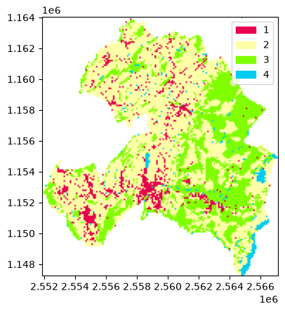
The Swiss Land Statistics (SLS) inventory distinguishes 27 land use/land cover classes, however, to simplify, this repository uses the classification aggregated into four main categories, i.e., urban (1), agricultural (3) wooded areas and (4) unproductive areas:
ls.plot_landscape(cmap=sls.noas04_4_cmap, norm=sls.noas04_4_norm, legend=True)
<Axes: >
Computing metrics#
The metrics can be computed at the patch, class and landscape level (see the list of implemented metrics)
Patch-level metrics#
The metrics can be computed at the patch level, that is, for each patch of the landscape:
patch_metrics_df = ls.compute_patch_metrics_df()
patch_metrics_df.head()
| class_val | area | perimeter | perimeter_area_ratio | shape_index | fractal_dimension | core_area | number_of_core_areas | core_area_index | euclidean_nearest_neighbor | |
|---|---|---|---|---|---|---|---|---|---|---|
| patch_id | ||||||||||
| 0 | 1 | 1.0 | 400.0 | 400.0 | 1.0 | 1.0 | 0.0 | 0 | 0.0 | 360.555128 |
| 1 | 1 | 1.0 | 400.0 | 400.0 | 1.0 | 1.0 | 0.0 | 0 | 0.0 | 360.555128 |
| 2 | 1 | 1.0 | 400.0 | 400.0 | 1.0 | 1.0 | 0.0 | 0 | 0.0 | 200.000000 |
| 3 | 1 | 1.0 | 400.0 | 400.0 | 1.0 | 1.0 | 0.0 | 0 | 0.0 | 200.000000 |
| 4 | 1 | 1.0 | 400.0 | 400.0 | 1.0 | 1.0 | 0.0 | 0 | 0.0 | 424.264069 |
We can operate upon patch_metrics_df as with any other pandas DataFrame. In this case, there are 206 patches, of which 193 are urban and 13 non-urban, as noted respectively by the values of 1 and 2 within the class_val column:
patch_metrics_df["class_val"].value_counts()
class_val
1    287
3    165
4    137
2     47
Name: count, dtype: int64
We might also use methods from other libraries, such as matplotlib or numpy. For instance, in order to explore the size distribution of patches, we can also plot the distribution of the logarithm of area for urban and agricultural classes as follows:
# for better-looking histograms
sns.set_theme()

ax = (
    patch_metrics_df[patch_metrics_df["class_val"] == URBAN_CLASS_VAL]
    .apply(np.log10)
    .hist(column="area", label="urban", density=True, alpha=0.66)
)
patch_metrics_df[patch_metrics_df["class_val"] == AGRICULTURAL_CLASS_VAL].apply(
    np.log10
).hist(column="area", ax=ax, label="agricultural", density=True, alpha=0.66)

ax.item().get_xaxis().set_major_formatter(
    mpl.ticker.FuncFormatter(lambda x, p: "10^%d" % x)
)
ax.item().legend()
<matplotlib.legend.Legend at 0x7f07bc5352b0>

ax = (
    patch_metrics_df[patch_metrics_df["class_val"] == 1]
    .apply(np.log10)
    .hist(column="area", label="urban", density=True)
)

Class-level metrics#
The metrics can also be computed at the class level, that is, aggregating over all patches of a land use/cover class
class_metrics_df = ls.compute_class_metrics_df()
class_metrics_df
| total_area | proportion_of_landscape | number_of_patches | patch_density | largest_patch_index | total_edge | edge_density | total_core_area | core_area_proportion_of_landscape | number_of_disjunct_core_areas | ... | euclidean_nearest_neighbor_md | euclidean_nearest_neighbor_ra | euclidean_nearest_neighbor_sd | euclidean_nearest_neighbor_cv | disjunct_core_area_mn | disjunct_core_area_am | disjunct_core_area_md | disjunct_core_area_ra | disjunct_core_area_sd | disjunct_core_area_cv | |
|---|---|---|---|---|---|---|---|---|---|---|---|---|---|---|---|---|---|---|---|---|---|
| class_val | |||||||||||||||||||||
| 1 | 1041.0 | 7.749572 | 287 | 2.136529 | 1.421872 | 256600.0 | 19.102211 | 90.0 | 0.669992 | 20 | ... | 223.606798 | 1100.000000 | 168.551251 | 54.504167 | 4.500000 | 20.400000 | 1.0 | 31.0 | 8.458723 | 187.971629 |
| 2 | 7907.0 | 58.862503 | 47 | 0.349885 | 46.862205 | 639500.0 | 47.606640 | 3589.0 | 26.717785 | 130 | ... | 200.000000 | 561.577311 | 84.548722 | 36.703367 | 27.607692 | 747.952354 | 3.0 | 1555.0 | 141.021466 | 510.804975 |
| 3 | 4126.0 | 30.715402 | 165 | 1.228318 | 20.605970 | 434600.0 | 32.353160 | 1636.0 | 12.178962 | 75 | ... | 223.606798 | 528.010989 | 94.721867 | 35.526380 | 21.813333 | 198.039120 | 3.0 | 395.0 | 62.000579 | 284.232484 |
| 4 | 359.0 | 2.672523 | 137 | 1.019876 | 0.588104 | 75900.0 | 5.650264 | 58.0 | 0.431773 | 8 | ... | 412.310563 | 3124.154028 | 381.220569 | 74.637981 | 7.250000 | 12.896552 | 5.5 | 20.0 | 6.398242 | 88.251613 |
4 rows × 66 columns
Landscape-level metrics#
Finally, the metrics can also be computed at the landscape level, that is, aggregating over all patches of the landscape
landscape_metrics_df = ls.compute_landscape_metrics_df()
landscape_metrics_df
| total_area | number_of_patches | patch_density | largest_patch_index | total_edge | edge_density | total_core_area | number_of_disjunct_core_areas | landscape_shape_index | effective_mesh_size | ... | euclidean_nearest_neighbor_md | euclidean_nearest_neighbor_ra | euclidean_nearest_neighbor_sd | euclidean_nearest_neighbor_cv | disjunct_core_area_mn | disjunct_core_area_am | disjunct_core_area_md | disjunct_core_area_ra | disjunct_core_area_sd | disjunct_core_area_cv | |
|---|---|---|---|---|---|---|---|---|---|---|---|---|---|---|---|---|---|---|---|---|---|
| 0 | 13433.0 | 636 | 4.734609 | 46.862205 | 703300.0 | 52.356138 | 5373.0 | 233 | 17.278017 | 3593.476141 | ... | 223.606798 | 3124.154028 | 236.550901 | 70.45117 | 23.060086 | 509.698816 | 3.0 | 1555.0 | 111.314332 | 482.7143 |
1 rows × 71 columns
Customizing the metrics DataFrames#
Selecting the metrics to compute#
Some metrics can be expensive to compute. If you are only interested in computing a subset of the metrics implemented within pylandstats, you can specify it in each respective method, that is, Landscape.compute_patch_metrics_df, Landscape.compute_patch_metrics_df and/or Landscape.compute_class_metrics_df through the metrics argument (see the documentation on “Computing metrics data frames”. For instance:
subset_class_metrics_df = ls.compute_class_metrics_df(
    metrics=["proportion_of_landscape", "edge_density"]
)
subset_class_metrics_df
| proportion_of_landscape | edge_density | |
|---|---|---|
| class_val | ||
| 1 | 7.749572 | 19.102211 |
| 2 | 58.862503 | 47.606640 |
| 3 | 30.715402 | 32.353160 |
| 4 | 2.672523 | 5.650264 |
Customizing how each metric is computed#
The default arguments correspond to how the metrics are defined within FRAGSTATS. Nevertheless, some metrics allow some variations in their definition. For instance, the edge_density above allows us to choose whether we consider the landscape boundary to be an edge (by default, as in FRAGSTATS, we do not, since we only consider edges between land use/cover classes), or whether we want the area to be converted to hectares (by default, as in FRAGSTATS, we do).
print(
    "Edge density (without boundary, meters of edge per hectare):\n{}\n".format(
        ls.edge_density()
    )
)

print(
    "Edge density (with boundary, meters of edge per hectare):\n{}\n".format(
        ls.edge_density(count_boundary=True)
    )
)

print(
    "Edge density (with boundary, meters of edge per square meter):\n{}".format(
        ls.edge_density(count_boundary=True, hectares=False)
    )
)
Edge density (without boundary, meters of edge per hectare):
52.35613786942604

Edge density (with boundary, meters of edge per hectare):
59.681381672001784

Edge density (with boundary, meters of edge per square meter):
0.005968138167200179
For more details, see the documentation for each metric’s method.
If we want to obtain a patch, class or landscape-level DataFrame with some customized metrics, instead of manually calling each metric’s method with its respective parameters, we can use the metrics_kwargs argument of the Landscape.compute_patch_metrics_df, Landscape.compute_patch_metrics_df and/or Landscape.compute_class_metrics_df to set the keyword arguments to be passed to the some metric methods. For instance, if we wanted proportion_of_landscape as a fraction instead of a percentage and edge_density to include the boundary, we can do it as follows:
custom_class_metrics_df = ls.compute_class_metrics_df(
    metrics_kwargs={
        "proportion_of_landscape": {"percent": False},
        "edge_density": {"count_boundary": True},
    }
)
custom_class_metrics_df
| total_area | proportion_of_landscape | number_of_patches | patch_density | largest_patch_index | total_edge | edge_density | total_core_area | core_area_proportion_of_landscape | number_of_disjunct_core_areas | ... | euclidean_nearest_neighbor_md | euclidean_nearest_neighbor_ra | euclidean_nearest_neighbor_sd | euclidean_nearest_neighbor_cv | disjunct_core_area_mn | disjunct_core_area_am | disjunct_core_area_md | disjunct_core_area_ra | disjunct_core_area_sd | disjunct_core_area_cv | |
|---|---|---|---|---|---|---|---|---|---|---|---|---|---|---|---|---|---|---|---|---|---|
| class_val | |||||||||||||||||||||
| 1 | 1041.0 | 0.077496 | 287 | 2.136529 | 1.421872 | 256600.0 | 19.325542 | 90.0 | 0.669992 | 20 | ... | 223.606798 | 1100.000000 | 168.551251 | 54.504167 | 4.500000 | 20.400000 | 1.0 | 31.0 | 8.458723 | 187.971629 |
| 2 | 7907.0 | 0.588625 | 47 | 0.349885 | 46.862205 | 639500.0 | 51.053376 | 3589.0 | 26.717785 | 130 | ... | 200.000000 | 561.577311 | 84.548722 | 36.703367 | 27.607692 | 747.952354 | 3.0 | 1555.0 | 141.021466 | 510.804975 |
| 3 | 4126.0 | 0.307154 | 165 | 1.228318 | 20.605970 | 434600.0 | 35.286235 | 1636.0 | 12.178962 | 75 | ... | 223.606798 | 528.010989 | 94.721867 | 35.526380 | 21.813333 | 198.039120 | 3.0 | 395.0 | 62.000579 | 284.232484 |
| 4 | 359.0 | 0.026725 | 137 | 1.019876 | 0.588104 | 75900.0 | 6.372367 | 58.0 | 0.431773 | 8 | ... | 412.310563 | 3124.154028 | 381.220569 | 74.637981 | 7.250000 | 12.896552 | 5.5 | 20.0 | 6.398242 | 88.251613 |
4 rows × 66 columns
Note that the values for proportion_of_landscape and edge_density are different now than when we computed them with the default arguments for their respective methods (in the class_metrics_df and subset_class_metrics_df above).
Note also that the custom_class_metrics_df does not only feature proportion_of_landscape and edge_density but features all the available metrics instead. This is because the metrics_kwargs argument does not imply that only the the metrics defined on it will be computed, only that the metrics defined on it will be computed with the specified arguments.
We might choose to only compute a reduced set of metrics, some of which with non-default arguments, by setting both the metrics and metric_kwargs arguments:
custom_subset_class_metrics_df = ls.compute_class_metrics_df(
    metrics=["proportion_of_landscape", "edge_density", "fractal_dimension_am"],
    metrics_kwargs={
        "proportion_of_landscape": {"percent": False},
        "edge_density": {"count_boundary": True},
    },
)
custom_subset_class_metrics_df
| proportion_of_landscape | edge_density | fractal_dimension_am | |
|---|---|---|---|
| class_val | |||
| 1 | 0.077496 | 19.325542 | 1.113777 |
| 2 | 0.588625 | 51.053376 | 1.284123 |
| 3 | 0.307154 | 35.286235 | 1.224259 |
| 4 | 0.026725 | 6.372367 | 1.058115 |
The same could be done for the Landscape.compute_patch_metrics_df or Landscape.compute_landscape_metrics_df methods. Check the documentation of each metric’s method for more details on how they might be customized through their arguments.