Spatial signature analysis

This notebook showcases the spatial signature analysis feature introduced in pylandstats v3.1.0. As an example use case, we explore an inventory of landscapes across the canton of Vaud (Switzerland), with the aim of characterizing them by means of their spatial signatures - namely a numerical embedding describing a landscape pattern. Examples of spatial signatures include a vector with the proportion of landscape occupied by each class, co-occurrence matrices reflecting pairwise adjacencies between classes or to vector of computed landscape metrics - see the motif R package and its journal article [1] for more details on spatial signatures.

Given a set of landscapes, their spatial signatures can be used to perform operations such as spatial pattern search, change detection or clustering (see Nowosad [1] for more details). In this example, spatial signatures are used to cluster landscapes and obtain a typology of Vaud landscapes. The cells of the data processing section serve to generate an inventory of local landscapes across the canton of Vaud. The landscape inventory is used to showcase how the SpatialSignatureAnalysis class can be used to explore the fundamental components of landscape metrics as well as to cluster landscapes. Finally, the landscape inventory is clustered using two types of spatial signatures, namely (a) a vector of ten recurrent landscape metrics and (b) an information theory (IT) approach based on Nowosad and Stepinski [2].

We will begin with some imports, definitions and data processing. If you are mainly interested in the features of SpatialSignatureAnalysis, feel free to skip to “2. Spatial signature analysis” section.

import geopandas as gpd
import matplotlib.pyplot as plt
import rasterio as rio
import seaborn as sns
import swisslandstats as sls
from rasterio import features
from shapely import geometry
from sklearn import decomposition

import pylandstats as pls

# set parameters which are not related to the cluster analysis itself (e.g., plotting)
# random seed to ensure repeatability of this notebook
random_seed = 0
# TODO: use random.PCG64 - see https://github.com/scikit-learn/scikit-learn/issues/16988
# bg = random.RandomState(random_seed)

# plotting parameters
figwidth, figheight = plt.rcParams["figure.figsize"]

heatmap_kwargs = dict(annot=True, fmt=".2f", cmap="coolwarm", vmin=-1, vmax=1)

# parameters for the cluster landscape plots
plot_cluster_landscapes_kwargs = dict(
    figsize=(3, 3),
    sample_kwargs=dict(random_state=random_seed),
    subfigures_kwargs=dict(hspace=0.05),
    supylabel_kwargs=dict(x=0.1),
    cmap=sls.noas04_4_cmap,
    norm=sls.noas04_4_norm,
)


def plot_cgram_eval(cgram, *, eval_methods=None):
    """Plot clustergram evaluation methods."""
    if eval_methods is None:
        eval_methods = [
            "silhouette_score",
            "calinski_harabasz_score",
            "davies_bouldin_score",
        ]
    n_plots = len(eval_methods)
    fig, axes = plt.subplots(n_plots, 1, figsize=(figwidth, figheight * n_plots))
    for eval_method, ax in zip(eval_methods, axes):
        getattr(cgram, eval_method)().plot(ax=ax)
        ax.set_ylabel(eval_method)

    ax.set_xlabel("n. clusters")

    return fig

1. Data preprocessing

The land use/land cover (LULC) data used in this notebook is a clip of the Swiss Land Statistics (SLS) survey over the canton of Vaud, which is shipped with the docs in the data/vaud directory. See the pylandstats-notebooks repository for the preprocessing pipeline that derives it from the raw SLS data.

We will set the main parameters of the cluster analysis in the cell below:

lulc_col = "LU18_4"
input_filepath = f"data/vaud/{lulc_col}.tif"

# Size (in meters) of each landscape, i.e., each landscape is a tile of 4000x4000 m^2,
# i.e., 4x4 km^2
landscape_size = 4000

Let us start by generating the landscapes for the spatial signature analysis by generating a ZonalGridAnalysis with the target grid size. However, in order to enhance landscape comparability, we will exclude the grid cells at the border of our raster extent so that we only have squared landscapes full of valid data pixels:

zga = pls.ZonalGridAnalysis(
    input_filepath,
    zone_width=landscape_size,
    zone_height=landscape_size,
    offset="center",
)
with rio.open(input_filepath) as src:
    extent_geom = gpd.GeoSeries(
        [
            geometry.shape(geom)
            for geom, val in features.shapes(
                src.dataset_mask(), transform=src.transform
            )
            if val != src.nodata
        ],
        crs=src.crs,
    ).union_all()

is_inner = zga.zone_gser.within(extent_geom)
ax = gpd.GeoDataFrame({"is_inner": is_inner}, geometry=zga.zone_gser).plot(
    column="is_inner", edgecolor="black", legend=True
)
for geom in extent_geom.geoms:
    ax.plot(*geom.exterior.xy, color="orange")

Let us now use the filtered geo-series of grid cells to instantiate a ZonalAnalysis with only the landscapes that are fully contained by the raster extent (i.e., the cantonal border):

za = pls.ZonalAnalysis(input_filepath, zga.zone_gser[is_inner].copy())

Here is what one of this landscapes looks like (legend: red pixels are urban, green pixels are agricultural, yellow pixels are wooded areas and blue pixels are unproductive areas, e.g., lakes, rivers, glaciers…):

za.landscape_ser.sample(1, random_state=random_seed).iloc[0].plot_landscape(
    cmap=sls.noas04_4_cmap, norm=sls.noas04_4_norm, legend=True
)

<Axes: >

Spatial signature analysis

We can now use the generated ZonalAnalysis instantiate the SpatialSignatureAnalysis class. In fact, we could also use any other pylandstats multi-landscape class (e.g., SpatioTemporalAnalysis, SpatioTemporalZonalAnalysis, ZonalGridAnalysis…). However, unlike the other pylandstats multi-landscape classes, in a SpatialSignatureAnalysis the metrics are computed when the object is instantiated. Therefore, the initialization requires the list of target metrics both for the class and landscape level:

ssa = pls.SpatialSignatureAnalysis(
    za,
    class_metrics=[
        "proportion_of_landscape",
        "edge_density",
    ],
    landscape_metrics=[
        "shannon_diversity_index",
    ],
)

[                                        ] | 0% Completed | 249.23 us

[####                                    ] | 11% Completed | 106.01 ms

[#########                               ] | 22% Completed | 209.99 ms

[#############                           ] | 33% Completed | 312.63 ms

[#################                       ] | 42% Completed | 503.01 ms

[#####################                   ] | 54% Completed | 611.85 ms

[##########################              ] | 65% Completed | 715.45 ms

[##############################          ] | 75% Completed | 817.81 ms

[###################################     ] | 88% Completed | 921.31 ms

[####################################### ] | 99% Completed | 1.02 s

[########################################] | 100% Completed | 1.12 s

[                                        ] | 0% Completed | 233.45 us

[#############                           ] | 33% Completed | 101.90 ms

[###########################             ] | 69% Completed | 205.72 ms

/home/docs/checkouts/readthedocs.org/user_builds/pylandstats/checkouts/latest/src/pylandstats/landscape.py:3572: RuntimeWarning: Entropy-based metrics can only be computed in landscapes with at least two classes of patches. Returning nan
  warnings.warn(

[########################################] | 100% Completed | 306.53 ms

The computed metrics for each landscape can be accessed via the metrics_df attribute, which is definitive and thus cannot be changed after the instantiation:

ssa.metrics_df.head()

	proportion_of_landscape_1	proportion_of_landscape_2	proportion_of_landscape_3	proportion_of_landscape_4	edge_density_1	edge_density_2	edge_density_3	edge_density_4	shannon_diversity_index
grid_cell
41	9.756098	46.097561	21.280488	22.865854	22.987805	29.817073	22.317073	6.585366	1.251045
81	4.085366	31.524390	64.268293	0.121951	11.890244	39.024390	33.597561	0.487805	0.780387
101	6.341463	47.987805	44.817073	0.853659	16.707317	44.024390	38.414634	3.292683	0.927724
102	5.853659	52.804878	40.670732	0.670732	16.646341	40.365854	29.878049	2.500000	0.900657
103	10.670732	66.585366	20.914634	1.829268	28.292683	46.707317	22.865854	5.182927	0.904777

As shown above, it is possible to include both metrics at the class and landscape level in the spatial signature by providing both the class_metrics and landscape_metrics arguments. Instead of using a multi-level index with the landscape id and class value (like in the other pylandstats multi-landscape classes), the class values are “pivoted” into the columns so that each row is a vector of metrics, i.e., the spatial signature of the landscape.

Therefore, the resulting data frame consists of a single row unique to each landscape, which features all the computed metrics (at the class and landscape-level) as columns, i.e., the spatial signature of the landscape.

Likewise the other pylandstats multi-landscape classes, we can use the classes argument compute the metrics for a subset of classes only. Similarly, it is possible to customize how the metrics are computed, however, in SpatialSignatureAnalysis.compute_metrics_df this is done by means of two arguments class_metrics_kwargs and landscape_metrics_kwargs, which customize the computation of the class and landscape-level metrics, respectively.

ssa = pls.SpatialSignatureAnalysis(
    za,
    class_metrics=[
        "proportion_of_landscape",
    ],
    classes=[1, 2],
    class_metrics_kwargs={"proportion_of_landscape": {"percent": False}},
    landscape_metrics=[
        "edge_density",
        "shannon_diversity_index",
    ],
    landscape_metrics_kwargs={
        "edge_density": {"count_boundary": True},
    },
)
ssa.metrics_df.head()

[                                        ] | 0% Completed | 201.36 us

[################################        ] | 80% Completed | 103.85 ms

[########################################] | 100% Completed | 204.64 ms

[                                        ] | 0% Completed | 204.79 us

[############                            ] | 31% Completed | 102.09 ms

[##########################              ] | 66% Completed | 207.28 ms

/home/docs/checkouts/readthedocs.org/user_builds/pylandstats/checkouts/latest/src/pylandstats/landscape.py:3572: RuntimeWarning: Entropy-based metrics can only be computed in landscapes with at least two classes of patches. Returning nan
  warnings.warn(

[########################################] | 100% Completed | 308.43 ms

	proportion_of_landscape_1	proportion_of_landscape_2	edge_density	shannon_diversity_index
grid_cell
41	0.097561	0.460976	50.731707	1.251045
81	0.040854	0.315244	52.378049	0.780387
101	0.063415	0.479878	61.097561	0.927724
102	0.058537	0.528049	54.573171	0.900657
103	0.106707	0.665854	61.402439	0.904777

Further details about the arguments of the SpatialSignatureAnalysis initialization can be found in the API documentation.

Let us now focus on the (many) potential applications of the spatial signature analysis. From a data science perspective, the metrics_df constitutes a dataset matrix in which each row is a sample (i.e., a landscape) that is in turn represented by a feature vector (i.e., a metric). This dataset matrix can be used for a wide range of computational landscape ecology applications, such as clustering similar landscapes or identifying the main components of spatial patterns [3]. In Python, the scikit-learn library [4] provides a wide range of tools for data science and machine learning that can be used for these purposes.

The sections below show how the SpatialSignatureAnalysis provides a convenient interface to use scikit-learn tools for clustering and component analysis of spatial patterns. Let us start by instantiating a SpatialSignatureAnalysis with the generated landscapes and a set of ten metrics (at the landscape level only) chosen loosely following the work of Nowosad and Stepinski [5] (the list of metrics is actually adapted considering the metrics that are currently implemented in pylandstats):

ten_metrics = [
    # area and edge
    "area_mn",
    "perimeter_mn",
    "patch_density",
    "edge_density",
    # shape
    "fractal_dimension_am",
    "shape_index_mn",
    # aggregation
    "contagion",
    "effective_mesh_size",
    "landscape_shape_index",
    # diversity
    "shannon_diversity_index",
]
ten_ssa = pls.SpatialSignatureAnalysis(
    za,
    landscape_metrics=ten_metrics,
)
ten_ssa.metrics_df.head()

[                                        ] | 0% Completed | 195.24 us

[##                                      ] | 5% Completed | 103.15 ms

[####                                    ] | 11% Completed | 215.72 ms

/home/docs/checkouts/readthedocs.org/user_builds/pylandstats/checkouts/latest/src/pylandstats/landscape.py:3636: RuntimeWarning: Entropy-based metrics can only be computed in landscapes with at least two classes of patches. Returning nan
  warnings.warn(
/home/docs/checkouts/readthedocs.org/user_builds/pylandstats/checkouts/latest/src/pylandstats/landscape.py:3572: RuntimeWarning: Entropy-based metrics can only be computed in landscapes with at least two classes of patches. Returning nan
  warnings.warn(

[######                                  ] | 16% Completed | 321.44 ms

[#########                               ] | 22% Completed | 436.50 ms

[###########                             ] | 27% Completed | 538.58 ms

[#############                           ] | 33% Completed | 642.10 ms

[###############                         ] | 38% Completed | 748.11 ms

[##################                      ] | 45% Completed | 859.62 ms

[####################                    ] | 51% Completed | 961.77 ms

[######################                  ] | 57% Completed | 1.07 s

[#########################               ] | 63% Completed | 1.18 s

/home/docs/checkouts/readthedocs.org/user_builds/pylandstats/checkouts/latest/src/pylandstats/landscape.py:3636: RuntimeWarning: Entropy-based metrics can only be computed in landscapes with at least two classes of patches. Returning nan
  warnings.warn(
/home/docs/checkouts/readthedocs.org/user_builds/pylandstats/checkouts/latest/src/pylandstats/landscape.py:3572: RuntimeWarning: Entropy-based metrics can only be computed in landscapes with at least two classes of patches. Returning nan
  warnings.warn(
/home/docs/checkouts/readthedocs.org/user_builds/pylandstats/checkouts/latest/src/pylandstats/landscape.py:3636: RuntimeWarning: Entropy-based metrics can only be computed in landscapes with at least two classes of patches. Returning nan
  warnings.warn(
/home/docs/checkouts/readthedocs.org/user_builds/pylandstats/checkouts/latest/src/pylandstats/landscape.py:3572: RuntimeWarning: Entropy-based metrics can only be computed in landscapes with at least two classes of patches. Returning nan
  warnings.warn(

[###########################             ] | 69% Completed | 1.29 s

[##############################          ] | 75% Completed | 1.39 s

/home/docs/checkouts/readthedocs.org/user_builds/pylandstats/checkouts/latest/src/pylandstats/landscape.py:3636: RuntimeWarning: Entropy-based metrics can only be computed in landscapes with at least two classes of patches. Returning nan
  warnings.warn(
/home/docs/checkouts/readthedocs.org/user_builds/pylandstats/checkouts/latest/src/pylandstats/landscape.py:3572: RuntimeWarning: Entropy-based metrics can only be computed in landscapes with at least two classes of patches. Returning nan
  warnings.warn(

[################################        ] | 81% Completed | 1.50 s

[##################################      ] | 86% Completed | 1.61 s

[#####################################   ] | 92% Completed | 1.71 s

[####################################### ] | 98% Completed | 1.82 s

[########################################] | 100% Completed | 1.92 s

	area_mn	perimeter_mn	patch_density	edge_density	fractal_dimension_am	shape_index_mn	contagion	effective_mesh_size	landscape_shape_index	shannon_diversity_index
grid_cell
41	22.465753	2057.534247	4.451220	40.853659	1.139659	1.245721	31.935570	446.415854	5.135802	1.251045
81	24.477612	2322.388060	4.085366	42.500000	1.162302	1.303821	51.064529	677.645122	5.302469	0.780387
101	21.298701	2392.207792	4.695122	51.219512	1.159822	1.308063	40.974428	282.596341	6.185185	0.927724
102	21.866667	2170.666667	4.573171	44.695122	1.155177	1.255156	44.602685	370.159756	5.524691	0.900657
103	16.907216	1909.278351	5.914634	51.524390	1.190591	1.222901	42.104588	758.135366	6.216049	0.904777

Component analysis

As extensively reviewed in the literature, landscape metrics are highly correlated, which can be problematic for many applications, e.g., multicolinearity can undermine statistical inference when establishing relationships between spatial pattern and ecological responses. Since metrics_df is a pandas data frame, we can easily compute the correlation matrix of the metrics and plot it as a heat map:

sns.heatmap(ten_ssa.metrics_df.corr(), **heatmap_kwargs)

<Axes: >

The heatmap shows that many metrics are almost perfectly correlated, either positively (e.g., edge density and landscape shape index) or negatively (e.g., contagion and Shannon diversity index).

One way to address this issue is to factorize the metrics data frame into a reduced set of components that explain the most variance in the data. To that end, the scikit-learn library features many classes implementing different decomposition algorithms. Let us use the Principal Component Analysis (PCA) algorithm:

# provide `random_state` for reproducibility
component_df, decompose_model = ten_ssa.decompose(
    decomposer=decomposition.PCA, random_state=random_seed
)
component_df.head()

/home/docs/checkouts/readthedocs.org/user_builds/pylandstats/checkouts/latest/src/pylandstats/spatial_signature.py:204: RuntimeWarning: The provided spatial signatures contain NaN values which are not supported by the decomposition model. In order to proceed, the NaN values will be dropped. However, you may consider either (i) changing the chosen metrics or (ii) imputing the NaN values by providing the `imputer` and `imputer_kwargs` arguments.
  warnings.warn(

	0	1	2	3	4	5	6	7	8	9
grid_cell
41	-0.918685	1.367801	-1.420042	-0.001153	0.638809	0.056352	0.008120	0.019208	0.029974	-4.855066e-15
81	0.924460	-0.089009	0.691759	-0.011045	-0.132987	0.124764	0.047324	-0.076973	0.010474	-6.422299e-15
101	-0.825088	0.529102	0.357993	-0.308471	-0.678712	-0.009435	-0.014827	-0.068802	-0.005666	-2.688568e-15
102	-0.068097	0.225409	-0.208567	-0.496494	-0.515389	0.079949	0.011733	-0.033704	0.007909	-3.294292e-15
103	-0.614859	-1.208682	-0.148580	0.189922	0.341966	0.046877	0.000259	0.041194	0.012082	-2.593801e-16

The decompose method returns both (i) a data frame with the components as columns and the landscapes as rows and (ii) the decomposition model. While the data frame alone may be hard to interpret, it can be used in conjunction with the decomposition model to obtain very useful information, such as the explained variance of each component and the loadings of each metric on each component.

We can access the explained variance of each component by using the explained_variance_ratio_ attribute of the decomposition model:

decompose_model.explained_variance_ratio_

array([6.49385636e-01, 1.73819954e-01, 1.25842607e-01, 2.40834511e-02,
       2.11916971e-02, 3.53708574e-03, 1.36814834e-03, 6.91267220e-04,
       8.01528184e-05, 0.00000000e+00])

As we can see, the four first components respectively explain a 64.94, 17.38, 12.58 and 2.41 % of the total variance (making it a total of 97.31 %). This information can be used to decide how many components to retain in the analysis.

We can also access the loadings of each metric on each component by using the get_loading_df method:

loading_df = ten_ssa.get_loading_df(decompose_model)
loading_df

	0	1	2	3	4	5	6	7	8	9
area_mn	0.028468	0.019172	0.006941	0.037736	-0.040639	-0.192460	-0.071242	0.298863	0.929657	-1.507409e-13
perimeter_mn	0.020465	0.111502	0.170472	-0.076747	0.036800	-0.244849	-0.073688	0.878146	-0.338115	1.139377e-13
patch_density	-0.347840	-0.433920	-0.213986	0.411313	-0.296756	0.537147	0.053885	0.310172	0.007148	1.584788e-14
edge_density	-0.396723	-0.198352	0.216409	0.105956	-0.144439	-0.436961	0.134602	-0.117570	-0.038341	-7.071068e-01
fractal_dimension_am	-0.272176	-0.372772	0.390417	-0.512837	0.504405	0.314704	0.060146	0.047280	0.110534	-1.772431e-14
shape_index_mn	-0.072102	0.481703	0.706428	0.388056	-0.048029	0.323786	0.029655	-0.047269	0.053648	-1.314434e-14
contagion	0.471247	-0.197188	0.168369	-0.082453	-0.230910	0.027691	0.802693	0.069175	0.026639	6.795756e-16
effective_mesh_size	0.326075	-0.351283	0.060949	0.607210	0.605275	-0.167212	-0.046077	-0.011421	-0.035861	5.800830e-15
landscape_shape_index	-0.396723	-0.198352	0.216409	0.105956	-0.144439	-0.436961	0.134602	-0.117570	-0.038341	7.071068e-01
shannon_diversity_index	-0.394111	0.432374	-0.384586	0.109371	0.436804	-0.002794	0.547192	0.079391	0.036510	-1.192839e-15

Given the explained variance, we can focus on the first four components and visualize this information using a heatmap:

# ten_ssa.plot_loading_heatmap(decompose_model)
n_components = 4
sns.heatmap(loading_df.iloc[:, :n_components], **heatmap_kwargs)

<Axes: >

As we can see, the first component is positively correlated with edge density and landscape shape index and negatively correlated with contagion, which suggest that this component is negatively related to the aggregation of patches. The second, third and fourth components are positively correlated with the mean shape index, area-weighted mean fractal dimension and mean patch area metrics.

In short, the component analysis can help identifying the fundamental components of spatial patterns and their relationships with the landscape metrics. This can help us in choosing the most relevant metrics for a given application and avoid multicolinearity issues.

Clustering landscapes based on spatial signatures

Another common application of the spatial signature analysis is to cluster similar landscapes based on their spatial patterns. To assist in this task, the SpatialSignatureAnalysis class provides a get_cgram method that computes a clustergram [6] based on the spatial signagures. The returned object is a Clustergram [7] instance that can be used to visualize clustergram diagrams and select the number of clusters:

# provide `random_state` for reproducibility
ten_cgram = ten_ssa.get_cgram(k_range=range(2, 10), random_state=random_seed)
ten_cgram.plot()

K=2 fitted in 0.060 seconds.
K=3 fitted in 0.003 seconds.
K=4 fitted in 0.002 seconds.
K=5 fitted in 0.002 seconds.
K=6 fitted in 0.002 seconds.
K=7 fitted in 0.002 seconds.
K=8 fitted in 0.002 seconds.
K=9 fitted in 0.003 seconds.

/home/docs/checkouts/readthedocs.org/user_builds/pylandstats/checkouts/latest/src/pylandstats/spatial_signature.py:353: RuntimeWarning: The provided spatial signatures contain NaN values which are not supported by the clustering model. In order to proceed, the NaN values will be dropped. However, you may consider either (i) changing the chosen metrics or (ii) imputing the NaN values by providing the `imputer` and `imputer_kwargs` arguments.
  warnings.warn(

<Axes: xlabel='Number of clusters (k)', ylabel='PCA weighted mean of the clusters'>

As we can see, setting the number of clusters to 3 seems a good choice. Alternatively, we can use the silhouette_score, calinski_harabasz_score and davies_bouldin_score methods of the returned cgram to evaluate the quality of the clustering for different numbers of clusters:

_ = plot_cgram_eval(ten_cgram)

Ideally, we want to pick the number of clusters that maximizes the silhouette_score and calinski_harabasz_score and minimizes the davies_bouldin_score, which in this case is in line with the clustergram diagram, i.e., 3 or 4 clusters.

Given the number of clusters, we can access the labels of the landscapes in each cluster by using the labels_ attribute of the cgram object:

n_clusters = 4
ten_cgram.labels_[n_clusters]

0      0
1      1
2      0
3      1
4      1
      ..
127    0
128    0
129    0
130    0
131    0
Name: 4, Length: 132, dtype: int32

We can also use scatterplot_cluster_metrics method of SpatialSignatureAnalysis to obtain a scatterplot of any given pair of metrics, with the landscapes colored by their cluster labels. Based on the metrics correlations and PCA loadings, we can choose the contagion, mean shape index, area-weighted mean fractal dimension and mean area metrics to visualize the clusters:

other_metrics = ["shape_index_mn", "fractal_dimension_am", "area_mn"]
fig, axes = plt.subplots(
    1,
    len(other_metrics),
    figsize=(len(other_metrics) * figwidth, figheight),
    sharey=True,
)
for other_metric, ax in zip(other_metrics, axes):
    ten_ssa.scatterplot_cluster_metrics(
        ten_cgram, n_clusters, other_metric, "contagion", ax=ax
    )

As we can see, the clusters can be largely separated by means of the contagion index only, with cluster “0” having low values, clusters “1” and “3” having mid-range values and cluster “2” having high values Additionally, clusters “2” and “3” are characterized by lower values of the area-weighted mean fractal dimension and higher values of mean patch area. Note that the colored “x” markers correspond to the centroids of their respective clusters.

To get a better grasp of the clustering results, we can use the plot_cluster_landscapes method to visualize the landscapes in each cluster:

ten_fig = ten_ssa.plot_cluster_landscapes(
    ten_cgram, n_clusters, **plot_cluster_landscapes_kwargs
)

Finally, we can use the plot_cluster_zones method to visualize the landscape extents colored by their cluster labels:

ten_ssa.plot_cluster_zones(ten_cgram, n_clusters)

<Axes: >

Note that we can only call plot_cluster_zones if the SpatialSignatureAnalysis instance has been initialized with a zonal analysis class (i.e., ZonalAnalysis, BufferAnalysis, ZonalGridAnalysis and their corresponding spatio-temporal analsysis classes).

Fundamental components of landscape patterns: further insights from information theory (IT)

The above sections illustrate how the SpatialSignatureAnalysis class operates with some example real-world applications. Let us now take this one step further and address a key question of spatial pattern analysis in landscape ecology (see the “Spatial patterns” section of the review of Hesselbarth et al. [3] for more details): what are the fundamental components of landscape configuration?

Following the approach of Nowosad and Stepinski [2], we will now try to use an information theory (IT)-based approach to classify landscapes, i.e., the HYU diagram, where H and U respectively refer to the Shannon’s entropy and the relative mutual information criterion (see Nowosad and Stepinski [2] for more details).

To perform this IT-based analysis, let us instantiate another SpatialSignatureAnalysis using these two metrics (which can only be computed at the landscape level):

it_metrics = ["entropy", "relative_mutual_information"]
it_ssa = pls.SpatialSignatureAnalysis(za, landscape_metrics=it_metrics)

[                                        ] | 0% Completed | 212.73 us

[###                                     ] | 8% Completed | 101.96 ms

[#######                                 ] | 19% Completed | 213.48 ms

[###########                             ] | 28% Completed | 323.04 ms

/home/docs/checkouts/readthedocs.org/user_builds/pylandstats/checkouts/latest/src/pylandstats/landscape.py:3572: RuntimeWarning: Entropy-based metrics can only be computed in landscapes with at least two classes of patches. Returning nan
  warnings.warn(
/home/docs/checkouts/readthedocs.org/user_builds/pylandstats/checkouts/latest/src/pylandstats/landscape.py:3636: RuntimeWarning: Entropy-based metrics can only be computed in landscapes with at least two classes of patches. Returning nan
  warnings.warn(

[###############                         ] | 37% Completed | 423.62 ms

[##################                      ] | 45% Completed | 527.70 ms

[######################                  ] | 55% Completed | 635.97 ms

[#########################               ] | 64% Completed | 743.08 ms

[#############################           ] | 72% Completed | 843.96 ms

[#################################       ] | 83% Completed | 961.46 ms

[#####################################   ] | 93% Completed | 1.07 s

[########################################] | 100% Completed | 1.18 s

Note that since we are only using two landscape metrics, we can skip the factorization into components (e.g., PCA) and proceed directly to the cluster analysis.

it_cgram = it_ssa.get_cgram(k_range=range(2, 10), random_state=random_seed)
it_cgram.plot()

K=2 fitted in 0.003 seconds.
K=3 fitted in 0.002 seconds.
K=4 fitted in 0.002 seconds.
K=5 fitted in 0.002 seconds.
K=6 fitted in 0.002 seconds.
K=7 fitted in 0.002 seconds.
K=8 fitted in 0.002 seconds.
K=9 fitted in 0.002 seconds.

/home/docs/checkouts/readthedocs.org/user_builds/pylandstats/checkouts/latest/src/pylandstats/spatial_signature.py:353: RuntimeWarning: The provided spatial signatures contain NaN values which are not supported by the clustering model. In order to proceed, the NaN values will be dropped. However, you may consider either (i) changing the chosen metrics or (ii) imputing the NaN values by providing the `imputer` and `imputer_kwargs` arguments.
  warnings.warn(

<Axes: xlabel='Number of clusters (k)', ylabel='PCA weighted mean of the clusters'>

Likewise the analysis based on ten landscape metrics, we can complement the clustergram with the other metrics:

_ = plot_cgram_eval(it_cgram)

The picture here is a bit more nuanced but the metrics seemingly agree that using 2 or 7 clusters is an appropriate choice. We can again visualize the clusters in a two-dimensional scatter plot of the two metrics:

n_clusters = 2
_ = it_ssa.scatterplot_cluster_metrics(
    it_cgram, n_clusters, "entropy", "relative_mutual_information"
)

It seems that the clusters can be linearly separated but in this case this requires considering the two metrics. Let us now visualize the landscapes of each cluster:

it_fig = it_ssa.plot_cluster_landscapes(
    it_cgram, n_clusters, **plot_cluster_landscapes_kwargs
)

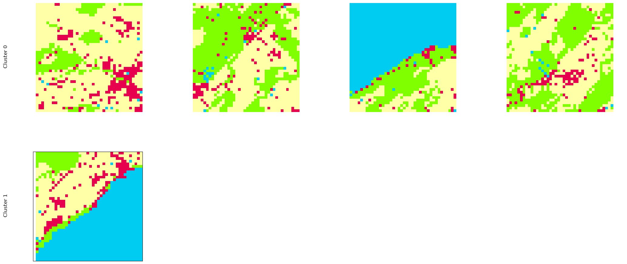
We can see that the cluster 1 seems to group the landscapes with most uneven distribution of class abundance (hence the lowest entropy values).

To conclude, let us compare the results of the ten metrics-based and the IT-based cluster analyses. We can evaluate the consistency of the ten metrics-based and the IT-based cluster classifications by comparing their respective silhouette scores:

colors = sns.color_palette()
fig, ax = plt.subplots()
for cgram, label, color in zip([ten_cgram, it_cgram], ["Ten metrics", "IT"], colors):
    cgram.silhouette_score().plot(color=color, ax=ax, label=label)
ax.legend()
ax.set_xlabel("n. clusters")
ax.set_ylabel("silhouette score")

Text(0, 0.5, 'silhouette score')

We can see that using ten metrics consistently results in lower silhouette scores than using the IT-based approach. Additionally, it is worth noting that using the ten metrics is very likely to result in multi-collinearity issues.

Finally, let us plot the landscape extents colored by their cluster labels on a map:

fig, axes = plt.subplots(1, 2, figsize=(figwidth * 2, figheight))
for ssa, cgram, title, ax in zip(
    [ten_ssa, it_ssa], [ten_cgram, it_cgram], ["Ten metrics", "IT"], axes
):
    ssa.plot_cluster_zones(cgram, n_clusters, ax=ax)
    ax.set_title(title)

Bonus track: spatial signatures in a spatio-temporal zonal analysis

Let us conclude by combining the spatial signatures with a spatio-temporal zonal analysis:

lulc_cols = ["LU85_4", "LU97_4", "LU09_4", "LU18_4"]
input_filepaths = [f"data/vaud/{lulc_col}.tif" for lulc_col in lulc_cols]
# note that these are the "survey" dates but each survey takes a total of 5 years so the
# actual date of each pixel depends on the region - see the "Swiss Land Use Statistics"
# documentation at https://shorturl.at/FMESv
dates = ["1985", "1997", "2009", "2018"]

stza = pls.SpatioTemporalZonalAnalysis(
    input_filepaths, zga.zone_gser[is_inner].copy(), dates=dates
)
stza_ssa = pls.SpatialSignatureAnalysis(stza, landscape_metrics=it_metrics)

[                                        ] | 0% Completed | 192.59 us

[                                        ] | 1% Completed | 104.71 ms

[#                                       ] | 3% Completed | 211.40 ms

[##                                      ] | 5% Completed | 314.40 ms

[##                                      ] | 7% Completed | 418.30 ms

[###                                     ] | 9% Completed | 523.46 ms

/home/docs/checkouts/readthedocs.org/user_builds/pylandstats/checkouts/latest/src/pylandstats/landscape.py:3572: RuntimeWarning: Entropy-based metrics can only be computed in landscapes with at least two classes of patches. Returning nan
  warnings.warn(
/home/docs/checkouts/readthedocs.org/user_builds/pylandstats/checkouts/latest/src/pylandstats/landscape.py:3636: RuntimeWarning: Entropy-based metrics can only be computed in landscapes with at least two classes of patches. Returning nan
  warnings.warn(

[####                                    ] | 11% Completed | 632.69 ms

[#####                                   ] | 13% Completed | 737.74 ms

[######                                  ] | 15% Completed | 844.08 ms

/home/docs/checkouts/readthedocs.org/user_builds/pylandstats/checkouts/latest/src/pylandstats/landscape.py:3572: RuntimeWarning: Entropy-based metrics can only be computed in landscapes with at least two classes of patches. Returning nan
  warnings.warn(
/home/docs/checkouts/readthedocs.org/user_builds/pylandstats/checkouts/latest/src/pylandstats/landscape.py:3636: RuntimeWarning: Entropy-based metrics can only be computed in landscapes with at least two classes of patches. Returning nan
  warnings.warn(

[######                                  ] | 16% Completed | 950.75 ms

[#######                                 ] | 19% Completed | 1.06 s

[########                                ] | 20% Completed | 1.16 s

[#########                               ] | 22% Completed | 1.27 s

[#########                               ] | 24% Completed | 1.37 s

[##########                              ] | 26% Completed | 1.48 s

[###########                             ] | 28% Completed | 1.58 s

[############                            ] | 30% Completed | 1.69 s

/home/docs/checkouts/readthedocs.org/user_builds/pylandstats/checkouts/latest/src/pylandstats/landscape.py:3572: RuntimeWarning: Entropy-based metrics can only be computed in landscapes with at least two classes of patches. Returning nan
  warnings.warn(
/home/docs/checkouts/readthedocs.org/user_builds/pylandstats/checkouts/latest/src/pylandstats/landscape.py:3636: RuntimeWarning: Entropy-based metrics can only be computed in landscapes with at least two classes of patches. Returning nan
  warnings.warn(
/home/docs/checkouts/readthedocs.org/user_builds/pylandstats/checkouts/latest/src/pylandstats/landscape.py:3572: RuntimeWarning: Entropy-based metrics can only be computed in landscapes with at least two classes of patches. Returning nan
  warnings.warn(
/home/docs/checkouts/readthedocs.org/user_builds/pylandstats/checkouts/latest/src/pylandstats/landscape.py:3636: RuntimeWarning: Entropy-based metrics can only be computed in landscapes with at least two classes of patches. Returning nan
  warnings.warn(
/home/docs/checkouts/readthedocs.org/user_builds/pylandstats/checkouts/latest/src/pylandstats/landscape.py:3572: RuntimeWarning: Entropy-based metrics can only be computed in landscapes with at least two classes of patches. Returning nan
  warnings.warn(
/home/docs/checkouts/readthedocs.org/user_builds/pylandstats/checkouts/latest/src/pylandstats/landscape.py:3636: RuntimeWarning: Entropy-based metrics can only be computed in landscapes with at least two classes of patches. Returning nan
  warnings.warn(

[############                            ] | 31% Completed | 1.86 s

[#############                           ] | 33% Completed | 1.97 s

/home/docs/checkouts/readthedocs.org/user_builds/pylandstats/checkouts/latest/src/pylandstats/landscape.py:3572: RuntimeWarning: Entropy-based metrics can only be computed in landscapes with at least two classes of patches. Returning nan
  warnings.warn(
/home/docs/checkouts/readthedocs.org/user_builds/pylandstats/checkouts/latest/src/pylandstats/landscape.py:3636: RuntimeWarning: Entropy-based metrics can only be computed in landscapes with at least two classes of patches. Returning nan
  warnings.warn(

[#############                           ] | 34% Completed | 2.08 s

[##############                          ] | 36% Completed | 2.18 s

[###############                         ] | 38% Completed | 2.29 s

/home/docs/checkouts/readthedocs.org/user_builds/pylandstats/checkouts/latest/src/pylandstats/landscape.py:3572: RuntimeWarning: Entropy-based metrics can only be computed in landscapes with at least two classes of patches. Returning nan
  warnings.warn(
/home/docs/checkouts/readthedocs.org/user_builds/pylandstats/checkouts/latest/src/pylandstats/landscape.py:3636: RuntimeWarning: Entropy-based metrics can only be computed in landscapes with at least two classes of patches. Returning nan
  warnings.warn(
/home/docs/checkouts/readthedocs.org/user_builds/pylandstats/checkouts/latest/src/pylandstats/landscape.py:3572: RuntimeWarning: Entropy-based metrics can only be computed in landscapes with at least two classes of patches. Returning nan
  warnings.warn(
/home/docs/checkouts/readthedocs.org/user_builds/pylandstats/checkouts/latest/src/pylandstats/landscape.py:3636: RuntimeWarning: Entropy-based metrics can only be computed in landscapes with at least two classes of patches. Returning nan
  warnings.warn(

[################                        ] | 40% Completed | 2.39 s

[#################                       ] | 42% Completed | 2.51 s

[#################                       ] | 44% Completed | 2.61 s

[##################                      ] | 46% Completed | 2.73 s

[###################                     ] | 48% Completed | 2.84 s

[####################                    ] | 50% Completed | 2.94 s

[#####################                   ] | 53% Completed | 3.05 s

[#####################                   ] | 54% Completed | 3.16 s

/home/docs/checkouts/readthedocs.org/user_builds/pylandstats/checkouts/latest/src/pylandstats/landscape.py:3572: RuntimeWarning: Entropy-based metrics can only be computed in landscapes with at least two classes of patches. Returning nan
  warnings.warn(
/home/docs/checkouts/readthedocs.org/user_builds/pylandstats/checkouts/latest/src/pylandstats/landscape.py:3636: RuntimeWarning: Entropy-based metrics can only be computed in landscapes with at least two classes of patches. Returning nan
  warnings.warn(
/home/docs/checkouts/readthedocs.org/user_builds/pylandstats/checkouts/latest/src/pylandstats/landscape.py:3572: RuntimeWarning: Entropy-based metrics can only be computed in landscapes with at least two classes of patches. Returning nan
  warnings.warn(
/home/docs/checkouts/readthedocs.org/user_builds/pylandstats/checkouts/latest/src/pylandstats/landscape.py:3636: RuntimeWarning: Entropy-based metrics can only be computed in landscapes with at least two classes of patches. Returning nan
  warnings.warn(
/home/docs/checkouts/readthedocs.org/user_builds/pylandstats/checkouts/latest/src/pylandstats/landscape.py:3572: RuntimeWarning: Entropy-based metrics can only be computed in landscapes with at least two classes of patches. Returning nan
  warnings.warn(
/home/docs/checkouts/readthedocs.org/user_builds/pylandstats/checkouts/latest/src/pylandstats/landscape.py:3636: RuntimeWarning: Entropy-based metrics can only be computed in landscapes with at least two classes of patches. Returning nan
  warnings.warn(

[######################                  ] | 56% Completed | 3.27 s

[#######################                 ] | 58% Completed | 3.37 s

[########################                ] | 60% Completed | 3.48 s

[#########################               ] | 62% Completed | 3.58 s

[#########################               ] | 64% Completed | 3.69 s

[##########################              ] | 66% Completed | 3.80 s

[###########################             ] | 68% Completed | 3.90 s

[############################            ] | 70% Completed | 4.01 s

[############################            ] | 72% Completed | 4.12 s

[#############################           ] | 74% Completed | 4.23 s

[##############################          ] | 75% Completed | 4.33 s

[###############################         ] | 77% Completed | 4.44 s

/home/docs/checkouts/readthedocs.org/user_builds/pylandstats/checkouts/latest/src/pylandstats/landscape.py:3572: RuntimeWarning: Entropy-based metrics can only be computed in landscapes with at least two classes of patches. Returning nan
  warnings.warn(
/home/docs/checkouts/readthedocs.org/user_builds/pylandstats/checkouts/latest/src/pylandstats/landscape.py:3636: RuntimeWarning: Entropy-based metrics can only be computed in landscapes with at least two classes of patches. Returning nan
  warnings.warn(

[###############################         ] | 79% Completed | 4.54 s

[################################        ] | 81% Completed | 4.65 s

[#################################       ] | 83% Completed | 4.75 s

[##################################      ] | 85% Completed | 4.85 s

/home/docs/checkouts/readthedocs.org/user_builds/pylandstats/checkouts/latest/src/pylandstats/landscape.py:3572: RuntimeWarning: Entropy-based metrics can only be computed in landscapes with at least two classes of patches. Returning nan
  warnings.warn(
/home/docs/checkouts/readthedocs.org/user_builds/pylandstats/checkouts/latest/src/pylandstats/landscape.py:3636: RuntimeWarning: Entropy-based metrics can only be computed in landscapes with at least two classes of patches. Returning nan
  warnings.warn(
/home/docs/checkouts/readthedocs.org/user_builds/pylandstats/checkouts/latest/src/pylandstats/landscape.py:3572: RuntimeWarning: Entropy-based metrics can only be computed in landscapes with at least two classes of patches. Returning nan
  warnings.warn(
/home/docs/checkouts/readthedocs.org/user_builds/pylandstats/checkouts/latest/src/pylandstats/landscape.py:3636: RuntimeWarning: Entropy-based metrics can only be computed in landscapes with at least two classes of patches. Returning nan
  warnings.warn(

[###################################     ] | 87% Completed | 4.96 s

[###################################     ] | 89% Completed | 5.06 s

[####################################    ] | 91% Completed | 5.16 s

[#####################################   ] | 93% Completed | 5.27 s

/home/docs/checkouts/readthedocs.org/user_builds/pylandstats/checkouts/latest/src/pylandstats/landscape.py:3572: RuntimeWarning: Entropy-based metrics can only be computed in landscapes with at least two classes of patches. Returning nan
  warnings.warn(
/home/docs/checkouts/readthedocs.org/user_builds/pylandstats/checkouts/latest/src/pylandstats/landscape.py:3636: RuntimeWarning: Entropy-based metrics can only be computed in landscapes with at least two classes of patches. Returning nan
  warnings.warn(

[######################################  ] | 95% Completed | 5.37 s

[######################################  ] | 97% Completed | 5.48 s

[####################################### ] | 99% Completed | 5.59 s

/home/docs/checkouts/readthedocs.org/user_builds/pylandstats/checkouts/latest/src/pylandstats/landscape.py:3572: RuntimeWarning: Entropy-based metrics can only be computed in landscapes with at least two classes of patches. Returning nan
  warnings.warn(
/home/docs/checkouts/readthedocs.org/user_builds/pylandstats/checkouts/latest/src/pylandstats/landscape.py:3636: RuntimeWarning: Entropy-based metrics can only be computed in landscapes with at least two classes of patches. Returning nan
  warnings.warn(

[########################################] | 100% Completed | 5.69 s

The SpatialSignatureAnalysis class work seamlessly, e.g., we can see the computed metrics (note that in this case, the landscapes are indexed by both the grid zone identifier and date):

stza_ssa.metrics_df

		entropy	relative_mutual_information
grid_cell	date
41	1985	1.735202	0.500226
	1997	1.757254	0.503210
	2009	1.774658	0.498169
	2018	1.804877	0.491544
81	1985	1.095977	0.270247
...	...	...	...
479	2018	1.302064	0.186902
502	1985	1.547218	0.356915
	1997	1.555701	0.359553
	2009	1.565866	0.374499
	2018	1.574006	0.356456

544 rows × 2 columns

We can also decompose the computed metrics into components as shown above, however it does not make sense since we are using the IT-based approach. Let us cluster the landscapes instead:

stza_cgram = stza_ssa.get_cgram(k_range=range(2, 10), random_state=random_seed)
stza_cgram.plot()
_ = plot_cgram_eval(stza_cgram)

/home/docs/checkouts/readthedocs.org/user_builds/pylandstats/checkouts/latest/src/pylandstats/spatial_signature.py:353: RuntimeWarning: The provided spatial signatures contain NaN values which are not supported by the clustering model. In order to proceed, the NaN values will be dropped. However, you may consider either (i) changing the chosen metrics or (ii) imputing the NaN values by providing the `imputer` and `imputer_kwargs` arguments.
  warnings.warn(

K=2 fitted in 0.002 seconds.
K=3 fitted in 0.002 seconds.
K=4 fitted in 0.003 seconds.
K=5 fitted in 0.002 seconds.
K=6 fitted in 0.003 seconds.
K=7 fitted in 0.002 seconds.
K=8 fitted in 0.003 seconds.
K=9 fitted in 0.003 seconds.

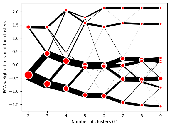
It seems that in this case considering 6 clusters can be more appropriate.

n_clusters = 6

Let us now plot the landscape clusters based on their metrics’ values:

_ = stza_ssa.scatterplot_cluster_metrics(
    stza_cgram, n_clusters, "entropy", "relative_mutual_information"
)

Again, the landscapes seem linearly separable when considering the two metrics.

Finally, the only difference when using a spatio-temporal zonal analysis class comes when plotting the cluster zones:

_ = stza_ssa.plot_cluster_zones(stza_cgram, n_clusters)

We can now visualize how the landscape clusters based on the IT metrics change over time.

Even though this is beyond the scope of this notebook, note that we have only included metrics of spatial configuration at the landscape level. Spatial abundance (namely the proportion of landscape metric at each class level) is certainly another fundamental component of spatial pattern, if not the most fundamental one [3, 5, 8-10]. In the IT-based approach, spatial abundance is likely reflected in the entropy metric, but it may be interesting to explicitly consider spatial abundance. Additionally, abundance of specific LULC classes can be a good predictor of many downstream applications.

References

1. Nowosad, Jakub. “Motif: an open-source R tool for pattern-based spatial analysis.” Landscape Ecology 36 (2021): 29-43.

2. Nowosad, J., & Stepinski, T. F. (2019). Information theory as a consistent framework for quantification and classification of landscape patterns. Landscape Ecology, 34(9), 2091-2101.

3. Hesselbarth, M. H., Nowosad, J., de Flamingh, A., Simpkins, C. E., Jung, M., Gerber, G., & Bosch, M. (2025). Computational Methods in Landscape Ecology. Current Landscape Ecology Reports, 10(1), 1-18.

4. Pedregosa, F., Varoquaux, G., Gramfort, A., Michel, V., Thirion, B., Grisel, O., … & Duchesnay, É. (2011). Scikit-learn: Machine learning in Python. the Journal of machine Learning research, 12, 2825-2830.

5. Nowosad, J., & Stepinski, T. F. (2018). Global inventory of landscape patterns and latent variables of landscape spatial configuration. Ecological Indicators, 89, 159-167.

6. Schonlau, M. (2002). The clustergram: A graph for visualizing hierarchical and nonhierarchical cluster analyses. The Stata Journal, 2(4), 391-402.

7. Fleischmann, M. (2023). Clustergram: Visualization and diagnostics for cluster analysis. Journal of Open Source Software, 8(89), 5240.

8. Gustafson, E. J. (1998). Quantifying landscape spatial pattern: what is the state of the art?. Ecosystems, 1(2), 143-156.

9. Gustafson, E. J. (2019). How has the state-of-the-art for quantification of landscape pattern advanced in the twenty-first century?. Landscape Ecology, 34, 2065-2072.

10. Riitters, K. (2019). Pattern metrics for a transdisciplinary landscape ecology. Landscape Ecology, 34(9), 2057-2063.