Spatio-temporal zonal analysis#
import contextily as cx
import geopandas as gpd
import matplotlib.pyplot as plt
from shapely.geometry import Point

import pylandstats as pls
In order to perform zonal analyses over time, pylandstats features an additional SpatioTemporalZonalAnalysis analysis class - as well as SpatioTemporalBufferAnalysis and SpatioTemporalZonalGridAnalysis.
Like in the spatio-temporal analysis example, we will use the three extracts of Veveyse district from the Swiss Land Statistics (SLS) datasets from the Swiss Federal Statistical Office for the years 1980, 1992, 2004 and 2013, yet in this case we also need to specify how the buffers are constructed.
The data used in this notebook ships with the docs in the data directory, namely:
the land use/land cover (LULC) data is downloaded and preprocessed (see A03-swisslandstats-preprocessing.ipynb for more details).
the elevation zones vector data is downloaded and preprocessed (see A04-elevation-zones.ipynb for more details).
Spatio-temporal zonal analysis#
Besides the base LULC maps, we will use a geopackage file defining a set of elevation zones. Like with the ZonalAnalysis class, we can use the zone_index argument to indicate which column of the geopackage file will be used to index the zones:
URBAN_CLASS_VAL = 1
input_filepaths = [
    "data/veveyse/LU85_4.tif",
    "data/veveyse/LU97_4.tif",
    "data/veveyse/LU09_4.tif",
    "data/veveyse/LU18_4.tif",
]
years = ["1980", "1992", "2004", "2013"]
elev_zones_filepath = "data/elev-zones.gpkg"

stza = pls.SpatioTemporalZonalAnalysis(
    input_filepaths, elev_zones_filepath, zone_index="elev-zone", dates=years
)
Like SpatioTemporalAnalysis, BufferAnalysis and/or ZonalAnalysis, we can compute the data frame of class metrics through the compute_class_metrics_df method:
class_metrics_df = stza.compute_class_metrics_df()
class_metrics_df.head()
[ ] | 0% Completed | 205.22 us
[ ] | 0% Completed | 115.12 ms
[ ] | 0% Completed | 258.09 ms
[ ] | 0% Completed | 368.82 ms
[### ] | 8% Completed | 474.93 ms
[###### ] | 16% Completed | 578.61 ms
/home/docs/checkouts/readthedocs.org/user_builds/pylandstats/checkouts/latest/.pixi/envs/doc/lib/python3.14/site-packages/numpy/_core/fromnumeric.py:3862: RuntimeWarning: Mean of empty slice
  return _methods._mean(a, axis=axis, dtype=dtype,
/home/docs/checkouts/readthedocs.org/user_builds/pylandstats/checkouts/latest/.pixi/envs/doc/lib/python3.14/site-packages/numpy/_core/_methods.py:142: RuntimeWarning: invalid value encountered in scalar divide
  ret = ret.dtype.type(ret / rcount)
/home/docs/checkouts/readthedocs.org/user_builds/pylandstats/checkouts/latest/src/pylandstats/landscape.py:776: SmallSampleWarning: One or more sample arguments is too small; all returned values will be NaN. See documentation for sample size requirements.
  return reduce_method(patch_metrics)
/home/docs/checkouts/readthedocs.org/user_builds/pylandstats/checkouts/latest/.pixi/envs/doc/lib/python3.14/site-packages/numpy/_core/fromnumeric.py:3862: RuntimeWarning: Mean of empty slice
  return _methods._mean(a, axis=axis, dtype=dtype,
/home/docs/checkouts/readthedocs.org/user_builds/pylandstats/checkouts/latest/.pixi/envs/doc/lib/python3.14/site-packages/numpy/_core/_methods.py:142: RuntimeWarning: invalid value encountered in scalar divide
  ret = ret.dtype.type(ret / rcount)
/home/docs/checkouts/readthedocs.org/user_builds/pylandstats/checkouts/latest/src/pylandstats/landscape.py:776: SmallSampleWarning: One or more sample arguments is too small; all returned values will be NaN. See documentation for sample size requirements.
  return reduce_method(patch_metrics)
[###### ] | 16% Completed | 719.55 ms
[###### ] | 16% Completed | 827.43 ms
[########## ] | 25% Completed | 928.50 ms
/home/docs/checkouts/readthedocs.org/user_builds/pylandstats/checkouts/latest/src/pylandstats/landscape.py:1324: RuntimeWarning: Class 1 has less than 2 patches. Euclidean-nearest-neighbor might contain nan values
  warnings.warn(
/home/docs/checkouts/readthedocs.org/user_builds/pylandstats/checkouts/latest/src/pylandstats/landscape.py:1324: RuntimeWarning: Class 1 has less than 2 patches. Euclidean-nearest-neighbor might contain nan values
  warnings.warn(
/home/docs/checkouts/readthedocs.org/user_builds/pylandstats/checkouts/latest/.pixi/envs/doc/lib/python3.14/site-packages/numpy/_core/fromnumeric.py:3862: RuntimeWarning: Mean of empty slice
  return _methods._mean(a, axis=axis, dtype=dtype,
/home/docs/checkouts/readthedocs.org/user_builds/pylandstats/checkouts/latest/.pixi/envs/doc/lib/python3.14/site-packages/numpy/_core/_methods.py:142: RuntimeWarning: invalid value encountered in scalar divide
  ret = ret.dtype.type(ret / rcount)
/home/docs/checkouts/readthedocs.org/user_builds/pylandstats/checkouts/latest/src/pylandstats/landscape.py:776: SmallSampleWarning: One or more sample arguments is too small; all returned values will be NaN. See documentation for sample size requirements.
  return reduce_method(patch_metrics)
[########## ] | 25% Completed | 1.06 s
[############# ] | 33% Completed | 1.17 s
[############# ] | 33% Completed | 1.33 s
[################ ] | 41% Completed | 1.44 s
[#################### ] | 50% Completed | 1.54 s
/home/docs/checkouts/readthedocs.org/user_builds/pylandstats/checkouts/latest/.pixi/envs/doc/lib/python3.14/site-packages/numpy/_core/fromnumeric.py:3862: RuntimeWarning: Mean of empty slice
  return _methods._mean(a, axis=axis, dtype=dtype,
/home/docs/checkouts/readthedocs.org/user_builds/pylandstats/checkouts/latest/.pixi/envs/doc/lib/python3.14/site-packages/numpy/_core/_methods.py:142: RuntimeWarning: invalid value encountered in scalar divide
  ret = ret.dtype.type(ret / rcount)
/home/docs/checkouts/readthedocs.org/user_builds/pylandstats/checkouts/latest/src/pylandstats/landscape.py:776: SmallSampleWarning: One or more sample arguments is too small; all returned values will be NaN. See documentation for sample size requirements.
  return reduce_method(patch_metrics)
[#################### ] | 50% Completed | 1.66 s
[#################### ] | 50% Completed | 1.76 s
[####################### ] | 58% Completed | 1.87 s
[####################### ] | 58% Completed | 1.98 s
/home/docs/checkouts/readthedocs.org/user_builds/pylandstats/checkouts/latest/.pixi/envs/doc/lib/python3.14/site-packages/numpy/_core/fromnumeric.py:3862: RuntimeWarning: Mean of empty slice
  return _methods._mean(a, axis=axis, dtype=dtype,
/home/docs/checkouts/readthedocs.org/user_builds/pylandstats/checkouts/latest/.pixi/envs/doc/lib/python3.14/site-packages/numpy/_core/_methods.py:142: RuntimeWarning: invalid value encountered in scalar divide
  ret = ret.dtype.type(ret / rcount)
/home/docs/checkouts/readthedocs.org/user_builds/pylandstats/checkouts/latest/src/pylandstats/landscape.py:776: SmallSampleWarning: One or more sample arguments is too small; all returned values will be NaN. See documentation for sample size requirements.
  return reduce_method(patch_metrics)
[########################## ] | 66% Completed | 2.08 s
[########################## ] | 66% Completed | 2.18 s
[############################## ] | 75% Completed | 2.28 s
/home/docs/checkouts/readthedocs.org/user_builds/pylandstats/checkouts/latest/.pixi/envs/doc/lib/python3.14/site-packages/numpy/_core/fromnumeric.py:3862: RuntimeWarning: Mean of empty slice
  return _methods._mean(a, axis=axis, dtype=dtype,
/home/docs/checkouts/readthedocs.org/user_builds/pylandstats/checkouts/latest/.pixi/envs/doc/lib/python3.14/site-packages/numpy/_core/_methods.py:142: RuntimeWarning: invalid value encountered in scalar divide
  ret = ret.dtype.type(ret / rcount)
/home/docs/checkouts/readthedocs.org/user_builds/pylandstats/checkouts/latest/src/pylandstats/landscape.py:776: SmallSampleWarning: One or more sample arguments is too small; all returned values will be NaN. See documentation for sample size requirements.
  return reduce_method(patch_metrics)
[############################## ] | 75% Completed | 2.40 s
[################################# ] | 83% Completed | 2.51 s
/home/docs/checkouts/readthedocs.org/user_builds/pylandstats/checkouts/latest/.pixi/envs/doc/lib/python3.14/site-packages/numpy/_core/fromnumeric.py:3862: RuntimeWarning: Mean of empty slice
  return _methods._mean(a, axis=axis, dtype=dtype,
/home/docs/checkouts/readthedocs.org/user_builds/pylandstats/checkouts/latest/.pixi/envs/doc/lib/python3.14/site-packages/numpy/_core/_methods.py:142: RuntimeWarning: invalid value encountered in scalar divide
  ret = ret.dtype.type(ret / rcount)
/home/docs/checkouts/readthedocs.org/user_builds/pylandstats/checkouts/latest/src/pylandstats/landscape.py:776: SmallSampleWarning: One or more sample arguments is too small; all returned values will be NaN. See documentation for sample size requirements.
  return reduce_method(patch_metrics)
[################################# ] | 83% Completed | 2.69 s
[########################################] | 100% Completed | 2.79 s
/home/docs/checkouts/readthedocs.org/user_builds/pylandstats/checkouts/latest/.pixi/envs/doc/lib/python3.14/site-packages/numpy/_core/fromnumeric.py:3862: RuntimeWarning: Mean of empty slice
  return _methods._mean(a, axis=axis, dtype=dtype,
/home/docs/checkouts/readthedocs.org/user_builds/pylandstats/checkouts/latest/.pixi/envs/doc/lib/python3.14/site-packages/numpy/_core/_methods.py:142: RuntimeWarning: invalid value encountered in scalar divide
  ret = ret.dtype.type(ret / rcount)
/home/docs/checkouts/readthedocs.org/user_builds/pylandstats/checkouts/latest/src/pylandstats/landscape.py:776: SmallSampleWarning: One or more sample arguments is too small; all returned values will be NaN. See documentation for sample size requirements.
  return reduce_method(patch_metrics)
| total_area | proportion_of_landscape | number_of_patches | patch_density | largest_patch_index | total_edge | edge_density | total_core_area | core_area_proportion_of_landscape | number_of_disjunct_core_areas | ... | euclidean_nearest_neighbor_md | euclidean_nearest_neighbor_ra | euclidean_nearest_neighbor_sd | euclidean_nearest_neighbor_cv | disjunct_core_area_mn | disjunct_core_area_am | disjunct_core_area_md | disjunct_core_area_ra | disjunct_core_area_sd | disjunct_core_area_cv | |||
|---|---|---|---|---|---|---|---|---|---|---|---|---|---|---|---|---|---|---|---|---|---|---|---|
| class_val | elev-zone | date | |||||||||||||||||||||
| 1 | <1000 | 1980 | 600.0 | 7.526342 | 253 | 3.173608 | 0.765178 | 175100.0 | 21.964375 | 24.0 | 0.301054 | 8 | ... | 223.606798 | 581.024968 | 120.302601 | 42.233561 | 3.000000 | 5.750000 | 2.0 | 9.0 | 2.872281 | 95.742711 |
| 1992 | 678.0 | 8.504767 | 253 | 3.173608 | 0.978424 | 190200.0 | 23.858505 | 27.0 | 0.338685 | 9 | ... | 223.606798 | 581.024968 | 109.769547 | 39.608538 | 3.000000 | 8.259259 | 1.0 | 13.0 | 3.972125 | 132.404170 | ||
| 2004 | 784.0 | 9.834420 | 252 | 3.161064 | 1.141495 | 204500.0 | 25.652283 | 48.0 | 0.602107 | 10 | ... | 223.606798 | 581.024968 | 107.584825 | 39.364455 | 4.800000 | 11.125000 | 2.5 | 16.0 | 5.509991 | 114.791478 | ||
| 2013 | 906.0 | 11.364777 | 235 | 2.947817 | 2.270447 | 218000.0 | 27.345710 | 87.0 | 1.091320 | 17 | ... | 223.606798 | 561.577311 | 104.264469 | 38.169258 | 5.117647 | 21.068966 | 1.0 | 31.0 | 9.035110 | 176.548132 | ||
| 1000-1500 | 1980 | 88.0 | 1.918047 | 44 | 0.959024 | 0.370532 | 27700.0 | 6.037489 | 1.0 | 0.021796 | 1 | ... | 300.000000 | 2616.025568 | 523.560381 | 106.374254 | 1.000000 | 1.000000 | 1.0 | 0.0 | 0.000000 | 0.000000 |
5 rows × 66 columns
Note that in this case, the data frame features a three-level MultiIndex that distinguishes the computed value for each class, zone and date. Again, we can operate upon such data frames as we would do with any other pandas data frame. For instance, we might want to evaluate the difference between the proportion of landscape occupied of urban patches (represented by a class_val of 1) computed for the elevation zone of “<1000” and “>1500”:
(
    class_metrics_df.loc[(1, "<1000"), "proportion_of_landscape"]
    - class_metrics_df.loc[(1, ">1500"), "proportion_of_landscape"]
)
date
1980     7.330647
1992     8.113377
2004     9.443031
2013    10.973387
Name: proportion_of_landscape, dtype: float64
Likewise in the other classes of pylandstats, if we want to compute the metrics data frame only for a subset of metrics or classes, or customize how the metrics are computed, we must respectively pass the arguments metrics, classes or metrics_kwargs to the compute_class_metrics_df and compute_landscape_metrics_df methods of SpatioTemporalZonalAnalysis as in:
metrics = ["proportion_of_landscape", "edge_density", "fractal_dimension_am"]
classes = [URBAN_CLASS_VAL]
metrics_kwargs = {
    "proportion_of_landscape": {"percent": False},
    "edge_density": {"count_boundary": True},
}
stza.compute_class_metrics_df(
    metrics=metrics, classes=classes, metrics_kwargs=metrics_kwargs
)
[ ] | 0% Completed | 164.98 us
[########################################] | 100% Completed | 101.11 ms
| proportion_of_landscape | edge_density | fractal_dimension_am | |||
|---|---|---|---|---|---|
| class_val | elev-zone | date | |||
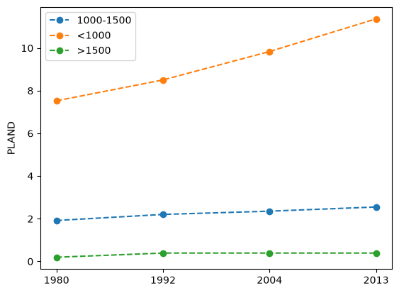
| 1 | <1000 | 1980 | 0.075263 | 22.353236 | 1.075028 |
| 1992 | 0.085048 | 24.284997 | 1.085124 | ||
| 2004 | 0.098344 | 26.141495 | 1.091537 | ||
| 2013 | 0.113648 | 27.872554 | 1.117441 | ||
| 1000-1500 | 1980 | 0.019180 | 6.146469 | 1.068200 | |
| 1992 | 0.022014 | 6.887533 | 1.067187 | ||
| 2004 | 0.023540 | 6.887533 | 1.069442 | ||
| 2013 | 0.025501 | 7.149085 | 1.068271 | ||
| >1500 | 1980 | 0.001957 | 0.782779 | 1.000000 | |
| 1992 | 0.003914 | 1.565558 | 1.000000 | ||
| 2004 | 0.003914 | 1.565558 | 1.000000 | ||
| 2013 | 0.003914 | 1.565558 | 1.000000 |
Another important functionality of the SpatioTemporalZonalAnalysis is plotting the time series of metrics at each zone. We can accomplish that through the plot_metric method. For instance, let us plot the proportion of landscape at the level of the urban class (class_val of 1):
stza.plot_metric("proportion_of_landscape", class_val=URBAN_CLASS_VAL)
[ ] | 0% Completed | 170.93 us
[########################################] | 100% Completed | 101.29 ms
<Axes: ylabel='PLAND'>
It can also be interesting to visualize such information in space by using compute_zonal_statistics_gdf method to obtain a geo-data frame:
zonal_statistics_gdf = stza.compute_zonal_statistics_gdf(
    metrics=metrics, class_val=URBAN_CLASS_VAL
)
zonal_statistics_gdf
[ ] | 0% Completed | 152.22 us
[########################################] | 100% Completed | 101.10 ms
| edge_density | fractal_dimension_am | proportion_of_landscape | geometry | ||||||||||
|---|---|---|---|---|---|---|---|---|---|---|---|---|---|
| date | 1980 | 1992 | 2004 | 2013 | 1980 | 1992 | 2004 | 2013 | 1980 | 1992 | 2004 | 2013 | |
| elev-zone | |||||||||||||
| 1000-1500 | 6.037489 | 6.734961 | 6.669573 | 6.931125 | 1.068200 | 1.067187 | 1.069442 | 1.068271 | 1.918047 | 2.201395 | 2.353967 | 2.550131 | POLYGON ((2563899.597 1160700.222, 2563899.594... |
| <1000 | 21.964375 | 23.858505 | 25.652283 | 27.345710 | 1.075028 | 1.085124 | 1.091537 | 1.117441 | 7.526342 | 8.504767 | 9.834420 | 11.364777 | MULTIPOLYGON (((2560899.573 1150500.318, 25606... |
| >1500 | 0.587084 | 1.369863 | 1.369863 | 1.369863 | 1.000000 | 1.000000 | 1.000000 | 1.000000 | 0.195695 | 0.391389 | 0.391389 | 0.391389 | MULTIPOLYGON (((2566299.561 1151500.225, 25664... |
Note that the columns of the geo-data frame are indexed in two levels, namely the metrics and dates. Since now we have a time series of values, we can spatially plot the evolution of the metrics at each zone:
num_years = len(years)
figwidth, figheight = plt.rcParams["figure.figsize"]
fig, axes = plt.subplots(1, num_years, figsize=(num_years * figwidth, figheight))

# get min and max values for all years to have the same scale across plots
vmin = zonal_statistics_gdf["proportion_of_landscape"].min().min()
vmax = zonal_statistics_gdf["proportion_of_landscape"].max().max()
for year, ax in zip(years, axes):
    zonal_statistics_gdf.plot(
        ("proportion_of_landscape", year),
        ax=ax,
        alpha=0.8,
        legend=True,
        vmin=vmin,
        vmax=vmax,
    )
    ax.set_title(year)
    cx.add_basemap(
        ax, crs=zonal_statistics_gdf.crs, source=cx.providers.CartoDB.Positron
    )

In fact, we can apply any transformation to the geo-data frame to visualize the metrics as required. For instance, we can transform the data frame to have separate columns for each year (how this is accomplished is beyond the scope of this tutorial), so that we can explore all the metrics values in the map:
plot_gdf = zonal_statistics_gdf.copy()  # drop("geometry", axis=1).unstack()
plot_gdf.columns = plot_gdf.columns.to_flat_index().map(lambda tup: "-".join(tup))
plot_gdf = gpd.GeoDataFrame(
    plot_gdf,
    geometry=plot_gdf.reset_index()["elev-zone"].map(stza.zone_gser).values,
    crs=stza.zone_gser.crs,
)
plot_gdf.explore()
Spatiotemporal buffer analysis#
Let us now consider three buffers of 2, 4 and 6km around the center of the town of Chatel-St-Denis. We can explore how landscape metrics at such extents change through times by using the SpatioTemporalBufferAnalysis class as in:
# latitude and longitude of the center of Chatel-St-Denis according to OpenStreetMap
base_geom = Point(6.8992073, 46.52634)
base_geom_crs = "+proj=longlat +ellps=WGS84 +datum=WGS84 +no_defs"

# buffer distances (in meters)
buffer_dists = [2000, 4000, 6000]

stba = pls.SpatioTemporalBufferAnalysis(
    input_filepaths, base_geom, buffer_dists, base_geom_crs=base_geom_crs, dates=years
)
Analogously to BufferAnalysis, we could also initialize the from a polygon geometry (such an administrative boundary) by passing such object as the base_geom argument. See the zonal analysis notebook to see how this can be done
The functionalities of SpatioTemporalBufferAnalysis are essentially the same as those of SpatioTemporalZonalAnalysis reviewed above:
class_metrics_df = stba.compute_class_metrics_df()
class_metrics_df.head()
[ ] | 0% Completed | 154.54 us
[ ] | 0% Completed | 139.35 ms
[ ] | 0% Completed | 253.48 ms
[ ] | 0% Completed | 375.37 ms
[### ] | 8% Completed | 480.74 ms
[###### ] | 16% Completed | 647.56 ms
[###### ] | 16% Completed | 769.33 ms
[########## ] | 25% Completed | 875.18 ms
[########## ] | 25% Completed | 991.79 ms
[############# ] | 33% Completed | 1.11 s
[############# ] | 33% Completed | 1.22 s
[############# ] | 33% Completed | 1.32 s
[#################### ] | 50% Completed | 1.43 s
[#################### ] | 50% Completed | 1.55 s
[#################### ] | 50% Completed | 1.72 s
[####################### ] | 58% Completed | 1.82 s
[####################### ] | 58% Completed | 1.94 s
[########################## ] | 66% Completed | 2.05 s
[############################## ] | 75% Completed | 2.19 s
[############################## ] | 75% Completed | 2.30 s
[################################# ] | 83% Completed | 2.45 s
[################################# ] | 83% Completed | 2.55 s
[#################################### ] | 91% Completed | 2.65 s
[########################################] | 100% Completed | 2.75 s
| total_area | proportion_of_landscape | number_of_patches | patch_density | largest_patch_index | total_edge | edge_density | total_core_area | core_area_proportion_of_landscape | number_of_disjunct_core_areas | ... | euclidean_nearest_neighbor_md | euclidean_nearest_neighbor_ra | euclidean_nearest_neighbor_sd | euclidean_nearest_neighbor_cv | disjunct_core_area_mn | disjunct_core_area_am | disjunct_core_area_md | disjunct_core_area_ra | disjunct_core_area_sd | disjunct_core_area_cv | |||
|---|---|---|---|---|---|---|---|---|---|---|---|---|---|---|---|---|---|---|---|---|---|---|---|
| class_val | buffer_dist | date | |||||||||||||||||||||
| 1 | 2000 | 1980 | 190.0 | 16.379310 | 38 | 3.275862 | 5.258621 | 41700.0 | 35.948276 | 16.0 | 1.379310 | 4 | ... | 223.606798 | 300.000000 | 93.295941 | 36.525402 | 4.000000 | 7.375000 | 2.5 | 9.0 | 3.674235 | 91.855865 |
| 1992 | 205.0 | 17.672414 | 38 | 3.275862 | 6.982759 | 45100.0 | 38.879310 | 20.0 | 1.724138 | 4 | ... | 223.606798 | 300.000000 | 87.204668 | 34.266810 | 5.000000 | 10.500000 | 2.5 | 13.0 | 5.244044 | 104.880885 | ||
| 2004 | 245.0 | 21.120690 | 34 | 2.931034 | 8.103448 | 48900.0 | 42.155172 | 29.0 | 2.500000 | 6 | ... | 211.803399 | 300.000000 | 73.176539 | 30.810177 | 4.833333 | 11.275862 | 3.0 | 16.0 | 5.580223 | 115.452890 | ||
| 2013 | 281.0 | 24.224138 | 25 | 2.155172 | 16.465517 | 50900.0 | 43.879310 | 45.0 | 3.879310 | 7 | ... | 223.606798 | 365.685425 | 98.258940 | 38.735937 | 6.428571 | 23.755556 | 1.0 | 31.0 | 10.554040 | 164.173952 | ||
| 4000 | 1980 | 308.0 | 8.358209 | 92 | 2.496608 | 1.655360 | 77700.0 | 21.085482 | 17.0 | 0.461330 | 5 | ... | 223.606798 | 581.024968 | 121.965405 | 44.023410 | 3.400000 | 7.000000 | 1.0 | 9.0 | 3.498571 | 102.899151 |
5 rows × 66 columns
stba.compute_landscape_metrics_df()
[ ] | 0% Completed | 149.27 us
[ ] | 0% Completed | 101.47 ms
[ ] | 0% Completed | 224.22 ms
[### ] | 8% Completed | 331.61 ms
[###### ] | 16% Completed | 435.01 ms
[########## ] | 25% Completed | 602.73 ms
[############# ] | 33% Completed | 705.71 ms
[############# ] | 33% Completed | 808.11 ms
[################ ] | 41% Completed | 914.76 ms
[#################### ] | 50% Completed | 1.05 s
[####################### ] | 58% Completed | 1.16 s
[########################## ] | 66% Completed | 1.30 s
[############################## ] | 75% Completed | 1.40 s
[############################## ] | 75% Completed | 1.50 s
[################################# ] | 83% Completed | 1.60 s
[#################################### ] | 91% Completed | 1.70 s
[########################################] | 100% Completed | 1.80 s
| total_area | number_of_patches | patch_density | largest_patch_index | total_edge | edge_density | total_core_area | number_of_disjunct_core_areas | landscape_shape_index | effective_mesh_size | ... | euclidean_nearest_neighbor_md | euclidean_nearest_neighbor_ra | euclidean_nearest_neighbor_sd | euclidean_nearest_neighbor_cv | disjunct_core_area_mn | disjunct_core_area_am | disjunct_core_area_md | disjunct_core_area_ra | disjunct_core_area_sd | disjunct_core_area_cv | ||
|---|---|---|---|---|---|---|---|---|---|---|---|---|---|---|---|---|---|---|---|---|---|---|
| buffer_dist | date | |||||||||||||||||||||
| 2000 | 1980 | 1160.0 | 85 | 7.327586 | 52.500000 | 71400.0 | 61.551724 | 344.0 | 32 | 6.492754 | 351.498276 | ... | 223.606798 | 507.106781 | 116.745726 | 41.547134 | 10.750000 | 93.827251 | 2.5 | 191.0 | 32.935543 | 306.377145 |
| 1992 | 1160.0 | 82 | 7.068966 | 51.551724 | 73300.0 | 63.189655 | 320.0 | 33 | 6.630435 | 341.605172 | ... | 223.606798 | 1134.166406 | 170.093612 | 56.477938 | 9.696970 | 84.192802 | 2.0 | 176.0 | 29.894243 | 308.284378 | |
| 2004 | 1160.0 | 81 | 6.982759 | 48.965517 | 76700.0 | 66.120690 | 292.0 | 38 | 6.876812 | 301.660345 | ... | 223.606798 | 1134.166406 | 167.444302 | 57.458152 | 7.684211 | 39.444444 | 2.0 | 97.0 | 17.873982 | 232.606612 | |
| 2013 | 1160.0 | 75 | 6.465517 | 46.206897 | 78800.0 | 67.931034 | 286.0 | 37 | 7.028986 | 294.739655 | ... | 223.606798 | 1134.166406 | 170.820531 | 57.576934 | 7.729730 | 35.434540 | 2.0 | 84.0 | 16.726171 | 216.387525 | |
| 4000 | 1980 | 3685.0 | 211 | 5.725916 | 51.804613 | 205500.0 | 55.766621 | 1307.0 | 73 | 10.012295 | 1054.102849 | ... | 223.606798 | 1242.220510 | 171.105182 | 55.994207 | 17.904110 | 209.228842 | 2.0 | 458.0 | 62.505269 | 349.111294 |
| 1992 | 3685.0 | 209 | 5.671642 | 51.316147 | 209200.0 | 56.770692 | 1280.0 | 75 | 10.163934 | 1050.495251 | ... | 223.606798 | 1242.220510 | 196.017807 | 62.120771 | 17.066667 | 248.021306 | 2.0 | 566.0 | 67.189946 | 393.691092 | |
| 2004 | 3685.0 | 199 | 5.400271 | 49.877883 | 213800.0 | 58.018996 | 1231.0 | 80 | 10.352459 | 989.770692 | ... | 223.606798 | 1242.220510 | 203.988269 | 63.479353 | 15.387500 | 181.107649 | 2.0 | 463.0 | 54.352666 | 353.226102 | |
| 2013 | 3685.0 | 188 | 5.101764 | 48.059701 | 218900.0 | 59.402985 | 1195.0 | 85 | 10.561475 | 932.959294 | ... | 223.606798 | 1242.220510 | 212.998332 | 65.499596 | 14.058824 | 142.385507 | 2.0 | 404.0 | 45.921507 | 326.638332 | |
| 6000 | 1980 | 7195.0 | 394 | 5.476025 | 53.787352 | 392900.0 | 54.607366 | 2680.0 | 123 | 13.426471 | 2200.019319 | ... | 223.606798 | 1100.000000 | 167.731726 | 54.134301 | 21.788618 | 346.469223 | 3.0 | 816.0 | 88.846012 | 407.763413 |
| 1992 | 7195.0 | 384 | 5.337040 | 52.008339 | 400300.0 | 55.635858 | 2601.0 | 138 | 13.644118 | 2117.035580 | ... | 223.606798 | 1036.931688 | 184.706512 | 58.616327 | 18.847826 | 333.688569 | 3.0 | 904.0 | 81.880781 | 434.430904 | |
| 2004 | 7195.0 | 367 | 5.100764 | 50.965949 | 402500.0 | 55.941626 | 2549.0 | 144 | 13.708824 | 2041.172620 | ... | 223.606798 | 1100.000000 | 203.675555 | 62.822660 | 17.701389 | 273.808333 | 3.0 | 796.0 | 71.813327 | 405.693175 | |
| 2013 | 7195.0 | 362 | 5.031272 | 49.478805 | 408200.0 | 56.733843 | 2500.0 | 151 | 13.876471 | 1938.907436 | ... | 223.606798 | 1276.482306 | 206.696588 | 63.575801 | 16.556291 | 145.835684 | 3.0 | 404.0 | 49.593398 | 299.544123 |
12 rows × 71 columns
Similarly, we can produce the same plot at the landscape level by omitting the class_val argument:
stba.plot_metric("fractal_dimension_am")
[ ] | 0% Completed | 138.97 us
[########################################] | 100% Completed | 101.30 ms
<Axes: ylabel='FRAC_AM'>

In this case, the legend shows the buffer distance that corresponds to the plotted line.
Spatiotemporal zonal grid analysis#
Finally, we can explore the temporal evolution of landscape metrics over a single regular rectangular grid using the SpatioTemporalZonalGridAnalysis class:
zone_width, zone_height = 2000, 2000  # in this case, in meters

stzga = pls.SpatioTemporalZonalGridAnalysis(
    input_filepaths, zone_width=zone_width, zone_height=zone_height, dates=years
)
Likewise with ZonalAnalysis we can also define the number of zones that we desire in each dimension by means of the num_zone_rows and num_zone_cols keyword arguments of the initialization method.
Again, the functionalities of SpatioTemporalZonalGridAnalysis are essentially the same as those of SpatioTemporalZonalAnalysis (and SpatioTemporalBufferAnalysis) reviewed above:
class_metrics_df = stzga.compute_class_metrics_df(metrics=metrics)
class_metrics_df.head()
[ ] | 0% Completed | 166.00 us
[## ] | 5% Completed | 108.57 ms
[### ] | 9% Completed | 220.52 ms
[##### ] | 14% Completed | 334.37 ms
[####### ] | 18% Completed | 436.43 ms
[######### ] | 23% Completed | 548.57 ms
[########### ] | 28% Completed | 650.75 ms
[############# ] | 33% Completed | 756.27 ms
[############### ] | 38% Completed | 863.73 ms
[################# ] | 42% Completed | 969.98 ms
[################### ] | 47% Completed | 1.07 s
[##################### ] | 52% Completed | 1.18 s
[####################### ] | 57% Completed | 1.29 s
[######################## ] | 62% Completed | 1.39 s
[########################## ] | 67% Completed | 1.50 s
[############################# ] | 72% Completed | 1.61 s
[############################## ] | 77% Completed | 1.72 s
[################################ ] | 82% Completed | 1.83 s
[################################## ] | 86% Completed | 1.93 s
[#################################### ] | 91% Completed | 2.04 s
[###################################### ] | 96% Completed | 2.14 s
[########################################] | 100% Completed | 2.25 s
| proportion_of_landscape | edge_density | fractal_dimension_am | |||
|---|---|---|---|---|---|
| class_val | grid_cell | date | |||
| 1 | 2 | 1980 | 8.241758 | 22.527473 | 1.018398 |
| 1992 | 9.340659 | 24.725275 | 1.057659 | ||
| 2004 | 9.890110 | 25.274725 | 1.063133 | ||
| 2013 | 12.087912 | 30.219780 | 1.081621 | ||
| 3 | 1980 | 1.801802 | 6.756757 | 1.034995 |