Overview of pylandstats#
import swisslandstats as sls

import pylandstats as pls
The data used in this notebook ships with the docs in the data directory, namely:
the land use/land cover (LULC) data (see A03-swisslandstats-preprocessing.ipynb for how it is derived from the raw SLS data).
the elevation zones vector data (see A04-elevation-zones.ipynb for more details).
Landscape analysis#
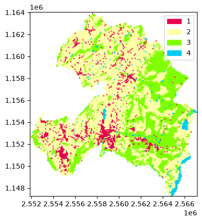
We can load landscapes from raster files and compute pandas data frames of patch, class and landscape level. See the notebook 01-landscape-analysis.ipynb for more thorough demonstration.
URBAN_CLASS_VAL = 1
input_filepath = "data/veveyse/LU18_4.tif"
ls = pls.Landscape(input_filepath)
ls.plot_landscape(cmap=sls.noas04_4_cmap, norm=sls.noas04_4_norm, legend=True)
<Axes: >
patch_metrics_df = ls.compute_patch_metrics_df()
patch_metrics_df.head()
| class_val | area | perimeter | perimeter_area_ratio | shape_index | fractal_dimension | core_area | number_of_core_areas | core_area_index | euclidean_nearest_neighbor | |
|---|---|---|---|---|---|---|---|---|---|---|
| patch_id | ||||||||||
| 0 | 1 | 1.0 | 400.0 | 400.0 | 1.0 | 1.0 | 0.0 | 0 | 0.0 | 360.555128 |
| 1 | 1 | 1.0 | 400.0 | 400.0 | 1.0 | 1.0 | 0.0 | 0 | 0.0 | 360.555128 |
| 2 | 1 | 1.0 | 400.0 | 400.0 | 1.0 | 1.0 | 0.0 | 0 | 0.0 | 200.000000 |
| 3 | 1 | 1.0 | 400.0 | 400.0 | 1.0 | 1.0 | 0.0 | 0 | 0.0 | 200.000000 |
| 4 | 1 | 1.0 | 400.0 | 400.0 | 1.0 | 1.0 | 0.0 | 0 | 0.0 | 424.264069 |
class_metrics_df = ls.compute_class_metrics_df()
class_metrics_df
| total_area | proportion_of_landscape | number_of_patches | patch_density | largest_patch_index | total_edge | edge_density | total_core_area | core_area_proportion_of_landscape | number_of_disjunct_core_areas | ... | euclidean_nearest_neighbor_md | euclidean_nearest_neighbor_ra | euclidean_nearest_neighbor_sd | euclidean_nearest_neighbor_cv | disjunct_core_area_mn | disjunct_core_area_am | disjunct_core_area_md | disjunct_core_area_ra | disjunct_core_area_sd | disjunct_core_area_cv | |
|---|---|---|---|---|---|---|---|---|---|---|---|---|---|---|---|---|---|---|---|---|---|
| class_val | |||||||||||||||||||||
| 1 | 1041.0 | 7.749572 | 287 | 2.136529 | 1.421872 | 256600.0 | 19.102211 | 90.0 | 0.669992 | 20 | ... | 223.606798 | 1100.000000 | 168.551251 | 54.504167 | 4.500000 | 20.400000 | 1.0 | 31.0 | 8.458723 | 187.971629 |
| 2 | 7907.0 | 58.862503 | 47 | 0.349885 | 46.862205 | 639500.0 | 47.606640 | 3589.0 | 26.717785 | 130 | ... | 200.000000 | 561.577311 | 84.548722 | 36.703367 | 27.607692 | 747.952354 | 3.0 | 1555.0 | 141.021466 | 510.804975 |
| 3 | 4126.0 | 30.715402 | 165 | 1.228318 | 20.605970 | 434600.0 | 32.353160 | 1636.0 | 12.178962 | 75 | ... | 223.606798 | 528.010989 | 94.721867 | 35.526380 | 21.813333 | 198.039120 | 3.0 | 395.0 | 62.000579 | 284.232484 |
| 4 | 359.0 | 2.672523 | 137 | 1.019876 | 0.588104 | 75900.0 | 5.650264 | 58.0 | 0.431773 | 8 | ... | 412.310563 | 3124.154028 | 381.220569 | 74.637981 | 7.250000 | 12.896552 | 5.5 | 20.0 | 6.398242 | 88.251613 |
4 rows × 66 columns
landscape_metrics_df = ls.compute_landscape_metrics_df()
landscape_metrics_df
| total_area | number_of_patches | patch_density | largest_patch_index | total_edge | edge_density | total_core_area | number_of_disjunct_core_areas | landscape_shape_index | effective_mesh_size | ... | euclidean_nearest_neighbor_md | euclidean_nearest_neighbor_ra | euclidean_nearest_neighbor_sd | euclidean_nearest_neighbor_cv | disjunct_core_area_mn | disjunct_core_area_am | disjunct_core_area_md | disjunct_core_area_ra | disjunct_core_area_sd | disjunct_core_area_cv | |
|---|---|---|---|---|---|---|---|---|---|---|---|---|---|---|---|---|---|---|---|---|---|
| 0 | 13433.0 | 636 | 4.734609 | 46.862205 | 703300.0 | 52.356138 | 5373.0 | 233 | 17.278017 | 3593.476141 | ... | 223.606798 | 3124.154028 | 236.550901 | 70.45117 | 23.060086 | 509.698816 | 3.0 | 1555.0 | 111.314332 | 482.7143 |
1 rows × 71 columns
Spatio-temporal analysis#
Given a temporally-ordered sequence of landscape snapshots, we can also analyze the spatio-temporal patterns of landscape change. To that end, pylandstats can compute pandas dataframes with the evolution of the metrics and plot them, both at the class and landscape level. See the notebook 02-spatiotemporal-analysis.ipynb for a more thorough demonstration.
input_filepaths = [
    "data/veveyse/LU85_4.tif",
    "data/veveyse/LU97_4.tif",
    "data/veveyse/LU09_4.tif",
    "data/veveyse/LU18_4.tif",
]
years = ["1980", "1992", "2004", "2013"]
sta = pls.SpatioTemporalAnalysis(input_filepaths, dates=years)
sta.compute_class_metrics_df()
[ ] | 0% Completed | 224.37 us
[ ] | 0% Completed | 104.86 ms
[ ] | 0% Completed | 221.05 ms
[ ] | 0% Completed | 344.06 ms
[ ] | 0% Completed | 468.63 ms
[ ] | 0% Completed | 574.43 ms
[ ] | 0% Completed | 676.61 ms
[ ] | 0% Completed | 780.06 ms
[ ] | 0% Completed | 886.85 ms
[#################### ] | 50% Completed | 987.85 ms
[#################### ] | 50% Completed | 1.10 s
[#################### ] | 50% Completed | 1.21 s
[#################### ] | 50% Completed | 1.31 s
[#################### ] | 50% Completed | 1.43 s
[#################### ] | 50% Completed | 1.53 s
[#################### ] | 50% Completed | 1.63 s
[#################### ] | 50% Completed | 1.73 s
[############################## ] | 75% Completed | 1.84 s
[########################################] | 100% Completed | 1.94 s
| total_area | proportion_of_landscape | number_of_patches | patch_density | largest_patch_index | total_edge | edge_density | total_core_area | core_area_proportion_of_landscape | number_of_disjunct_core_areas | ... | euclidean_nearest_neighbor_md | euclidean_nearest_neighbor_ra | euclidean_nearest_neighbor_sd | euclidean_nearest_neighbor_cv | disjunct_core_area_mn | disjunct_core_area_am | disjunct_core_area_md | disjunct_core_area_ra | disjunct_core_area_sd | disjunct_core_area_cv | ||
|---|---|---|---|---|---|---|---|---|---|---|---|---|---|---|---|---|---|---|---|---|---|---|
| class_val | dates | |||||||||||||||||||||
| 1 | 1980 | 702.0 | 5.225936 | 304 | 2.263083 | 0.454106 | 208400.0 | 15.514033 | 25.0 | 0.186109 | 9 | ... | 223.606798 | 1100.000000 | 169.300811 | 55.094159 | 2.777778 | 5.560000 | 1.0 | 9.0 | 2.779999 | 100.079968 |
| 1992 | 794.0 | 5.910817 | 309 | 2.300305 | 0.602993 | 227800.0 | 16.958237 | 28.0 | 0.208442 | 10 | ... | 223.606798 | 940.175425 | 156.817097 | 52.299458 | 2.800000 | 8.000000 | 1.0 | 13.0 | 3.815757 | 136.277029 | |
| 2004 | 906.0 | 6.744584 | 304 | 2.263083 | 0.699769 | 242000.0 | 18.015335 | 50.0 | 0.372218 | 12 | ... | 223.606798 | 1100.000000 | 162.962720 | 54.136494 | 4.166667 | 10.720000 | 1.5 | 16.0 | 5.225472 | 125.411323 | |
| 2013 | 1041.0 | 7.749572 | 287 | 2.136529 | 1.421872 | 256600.0 | 19.102211 | 90.0 | 0.669992 | 20 | ... | 223.606798 | 1100.000000 | 168.551251 | 54.504167 | 4.500000 | 20.400000 | 1.0 | 31.0 | 8.458723 | 187.971629 | |
| 2 | 1980 | 8351.0 | 62.167796 | 32 | 0.238219 | 52.170029 | 615000.0 | 45.782774 | 4076.0 | 30.343185 | 107 | ... | 200.000000 | 470.820393 | 85.842455 | 36.252869 | 38.093458 | 740.707066 | 3.0 | 1352.0 | 163.600067 | 429.470245 |
| 1992 | 8185.0 | 60.932033 | 40 | 0.297774 | 48.596739 | 621700.0 | 46.281545 | 3902.0 | 29.047867 | 116 | ... | 200.000000 | 561.577311 | 92.279333 | 38.656807 | 33.637931 | 754.402358 | 3.0 | 1444.0 | 155.708137 | 462.894514 | |
| 2004 | 8052.0 | 59.941934 | 42 | 0.312663 | 47.829971 | 630500.0 | 46.936649 | 3735.0 | 27.804660 | 123 | ... | 200.000000 | 561.577311 | 88.608659 | 37.780919 | 30.365854 | 1162.704953 | 3.0 | 2049.0 | 185.430427 | 610.654419 | |
| 2013 | 7907.0 | 58.862503 | 47 | 0.349885 | 46.862205 | 639500.0 | 47.606640 | 3589.0 | 26.717785 | 130 | ... | 200.000000 | 561.577311 | 84.548722 | 36.703367 | 27.607692 | 747.952354 | 3.0 | 1555.0 | 141.021466 | 510.804975 | |
| 3 | 1980 | 3967.0 | 29.531750 | 169 | 1.258096 | 15.610809 | 438500.0 | 32.643490 | 1509.0 | 11.233529 | 76 | ... | 223.606798 | 408.276253 | 89.161532 | 34.170355 | 19.855263 | 171.243870 | 4.5 | 360.0 | 54.825730 | 276.126935 |
| 1992 | 4072.0 | 30.313407 | 161 | 1.198541 | 18.573662 | 439500.0 | 32.717933 | 1584.0 | 11.791856 | 76 | ... | 223.606798 | 408.276253 | 89.394894 | 33.994777 | 20.842105 | 187.746212 | 3.5 | 386.0 | 58.979937 | 282.984546 | |
| 2004 | 4112.0 | 30.611181 | 162 | 1.205985 | 20.576193 | 434300.0 | 32.330827 | 1633.0 | 12.156629 | 76 | ... | 223.606798 | 528.010989 | 95.923385 | 36.129383 | 21.486842 | 192.037355 | 3.0 | 395.0 | 60.535873 | 281.734621 | |
| 2013 | 4126.0 | 30.715402 | 165 | 1.228318 | 20.605970 | 434600.0 | 32.353160 | 1636.0 | 12.178962 | 75 | ... | 223.606798 | 528.010989 | 94.721867 | 35.526380 | 21.813333 | 198.039120 | 3.0 | 395.0 | 62.000579 | 284.232484 | |
| 4 | 1980 | 413.0 | 3.074518 | 161 | 1.198541 | 0.580660 | 92100.0 | 6.856250 | 57.0 | 0.424328 | 8 | ... | 360.555128 | 3124.154028 | 330.484033 | 74.180497 | 7.125000 | 12.403509 | 6.0 | 18.0 | 6.132648 | 86.072257 |
| 1992 | 382.0 | 2.843743 | 152 | 1.131542 | 0.595548 | 83000.0 | 6.178813 | 58.0 | 0.431773 | 7 | ... | 400.000000 | 3124.154028 | 352.800892 | 74.148800 | 8.285714 | 13.551724 | 9.0 | 18.0 | 6.605502 | 79.721573 | |
| 2004 | 363.0 | 2.702300 | 144 | 1.071987 | 0.580660 | 76000.0 | 5.657709 | 58.0 | 0.431773 | 8 | ... | 412.310563 | 3124.154028 | 366.682284 | 72.359808 | 7.250000 | 12.896552 | 5.5 | 20.0 | 6.398242 | 88.251613 | |
| 2013 | 359.0 | 2.672523 | 137 | 1.019876 | 0.588104 | 75900.0 | 5.650264 | 58.0 | 0.431773 | 8 | ... | 412.310563 | 3124.154028 | 381.220569 | 74.637981 | 7.250000 | 12.896552 | 5.5 | 20.0 | 6.398242 | 88.251613 |
16 rows × 66 columns
sta.compute_landscape_metrics_df()
[ ] | 0% Completed | 146.21 us
[ ] | 0% Completed | 108.64 ms
[ ] | 0% Completed | 211.92 ms
[ ] | 0% Completed | 314.41 ms
[#################### ] | 50% Completed | 421.58 ms
[#################### ] | 50% Completed | 523.05 ms
[#################### ] | 50% Completed | 629.62 ms
[#################### ] | 50% Completed | 736.34 ms
[########################################] | 100% Completed | 845.10 ms
| total_area | number_of_patches | patch_density | largest_patch_index | total_edge | edge_density | total_core_area | number_of_disjunct_core_areas | landscape_shape_index | effective_mesh_size | ... | euclidean_nearest_neighbor_md | euclidean_nearest_neighbor_ra | euclidean_nearest_neighbor_sd | euclidean_nearest_neighbor_cv | disjunct_core_area_mn | disjunct_core_area_am | disjunct_core_area_md | disjunct_core_area_ra | disjunct_core_area_sd | disjunct_core_area_cv | |
|---|---|---|---|---|---|---|---|---|---|---|---|---|---|---|---|---|---|---|---|---|---|
| dates | |||||||||||||||||||||
| 1980 | 13433.0 | 666 | 4.957939 | 52.170029 | 677000.0 | 50.398273 | 5667.0 | 200 | 16.711207 | 4074.760143 | ... | 223.606798 | 3124.154028 | 216.625926 | 66.540480 | 28.335000 | 533.272195 | 3.0 | 1352.0 | 124.855928 | 440.642061 |
| 1992 | 13433.0 | 662 | 4.928162 | 48.596739 | 686000.0 | 51.068265 | 5572.0 | 209 | 16.905172 | 3721.028140 | ... | 223.606798 | 3124.154028 | 222.286812 | 67.856637 | 26.660287 | 534.324217 | 3.0 | 1444.0 | 121.661679 | 456.340467 |
| 2004 | 13433.0 | 652 | 4.853718 | 47.829971 | 691400.0 | 51.470260 | 5476.0 | 219 | 17.021552 | 3711.910593 | ... | 223.606798 | 3124.154028 | 231.885409 | 69.562278 | 25.004566 | 777.260594 | 3.0 | 2049.0 | 143.674210 | 574.591890 |
| 2013 | 13433.0 | 636 | 4.734609 | 46.862205 | 703300.0 | 52.356138 | 5373.0 | 233 | 17.278017 | 3593.476141 | ... | 223.606798 | 3124.154028 | 236.550901 | 70.451170 | 23.060086 | 509.698816 | 3.0 | 1555.0 | 111.314332 | 482.714300 |
4 rows × 71 columns
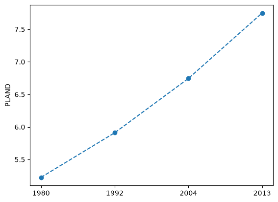
We can also plot the time series of metrics at the class level, e.g., the evolution of the proportion of landscape occupied by the land use class value 1 (urban):
sta.plot_metric("proportion_of_landscape", class_val=URBAN_CLASS_VAL)
[ ] | 0% Completed | 133.87 us
[########################################] | 100% Completed | 100.97 ms
<Axes: ylabel='PLAND'>
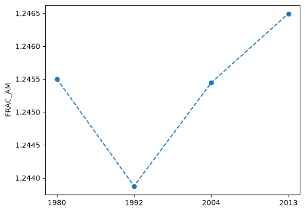
or we can also plot at the landscape level by not providing any class_val argument, e.g., the evolution of the area-weighted mean fractal dimension of all the patches of the landscape:
sta.plot_metric("fractal_dimension_am")
[ ] | 0% Completed | 149.21 us
[########################################] | 100% Completed | 101.14 ms
<Axes: ylabel='FRAC_AM'>
Zonal analysis#
Zonal analysis is a common procedure to compute statistics for a set of specified spatial zones. PyLandStats features three classes to perform zonal analysis, ZonalAnalysis, BufferAnalysis and ZonalGridAnalysis. The first allows user to fully customize how the zones are defined, while BufferAnalysis and ZonalGriAnalysis provide a convenient way to instantiate specific cases of zonal analysis, i.e., adding buffers around a feature of interest or as a regular rectangular grid over the landscape, respectively. See the notebook 03-zonal-analysis.ipynb for a thorough demonstration of the use cases described above.
To define the zones of a ZonalAnalysis, we can use - among other options - any geographic data file that can be read by geopandas.read_file. For instance, we can use a geopackage file defining three elevation zones in our landscape:
elev_zones_filepath = "data/elev-zones.gpkg"

za = pls.ZonalAnalysis(input_filepath, elev_zones_filepath, zone_index="elev-zone")
# plot the landscapes of each zone
fig = za.plot_landscapes(
    cmap=sls.noas04_4_cmap, show_kwargs=dict(norm=sls.noas04_4_norm)
)
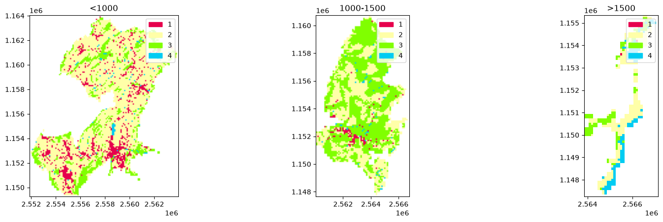
Analogously to the spatio-temporal analysis, we can use the compute_class_metrics_df and compute_landscape_metrics_df methods to compute the metrics for each zone:
za.compute_class_metrics_df()
[ ] | 0% Completed | 136.89 us
[ ] | 0% Completed | 101.56 ms
[ ] | 0% Completed | 237.63 ms
[############# ] | 33% Completed | 402.97 ms
[############# ] | 33% Completed | 518.33 ms
/home/docs/checkouts/readthedocs.org/user_builds/pylandstats/checkouts/latest/.pixi/envs/doc/lib/python3.14/site-packages/numpy/_core/fromnumeric.py:3862: RuntimeWarning: Mean of empty slice
  return _methods._mean(a, axis=axis, dtype=dtype,
/home/docs/checkouts/readthedocs.org/user_builds/pylandstats/checkouts/latest/.pixi/envs/doc/lib/python3.14/site-packages/numpy/_core/_methods.py:142: RuntimeWarning: invalid value encountered in scalar divide
  ret = ret.dtype.type(ret / rcount)
/home/docs/checkouts/readthedocs.org/user_builds/pylandstats/checkouts/latest/src/pylandstats/landscape.py:737: SmallSampleWarning: One or more sample arguments is too small; all returned values will be NaN. See documentation for sample size requirements.
  return reduce_method(patch_metrics)
[############# ] | 33% Completed | 639.34 ms
[########################## ] | 66% Completed | 740.54 ms
[########################################] | 100% Completed | 841.63 ms
/home/docs/checkouts/readthedocs.org/user_builds/pylandstats/checkouts/latest/.pixi/envs/doc/lib/python3.14/site-packages/numpy/_core/fromnumeric.py:3862: RuntimeWarning: Mean of empty slice
  return _methods._mean(a, axis=axis, dtype=dtype,
/home/docs/checkouts/readthedocs.org/user_builds/pylandstats/checkouts/latest/.pixi/envs/doc/lib/python3.14/site-packages/numpy/_core/_methods.py:142: RuntimeWarning: invalid value encountered in scalar divide
  ret = ret.dtype.type(ret / rcount)
/home/docs/checkouts/readthedocs.org/user_builds/pylandstats/checkouts/latest/src/pylandstats/landscape.py:737: SmallSampleWarning: One or more sample arguments is too small; all returned values will be NaN. See documentation for sample size requirements.
  return reduce_method(patch_metrics)
| total_area | proportion_of_landscape | number_of_patches | patch_density | largest_patch_index | total_edge | edge_density | total_core_area | core_area_proportion_of_landscape | number_of_disjunct_core_areas | ... | euclidean_nearest_neighbor_md | euclidean_nearest_neighbor_ra | euclidean_nearest_neighbor_sd | euclidean_nearest_neighbor_cv | disjunct_core_area_mn | disjunct_core_area_am | disjunct_core_area_md | disjunct_core_area_ra | disjunct_core_area_sd | disjunct_core_area_cv | ||
|---|---|---|---|---|---|---|---|---|---|---|---|---|---|---|---|---|---|---|---|---|---|---|
| class_val | elev-zone | |||||||||||||||||||||
| 1 | <1000 | 906.0 | 11.364777 | 235 | 2.947817 | 2.270447 | 218000.0 | 27.345710 | 87.0 | 1.091320 | 17 | ... | 223.606798 | 561.577311 | 104.264469 | 38.169258 | 5.117647 | 21.068966 | 1.0 | 31.0 | 9.035110 | 176.548132 |
| 1000-1500 | 117.0 | 2.550131 | 48 | 1.046207 | 0.457716 | 31800.0 | 6.931125 | 2.0 | 0.043592 | 2 | ... | 360.555128 | 2216.609195 | 439.448544 | 90.250243 | 1.000000 | 1.000000 | 1.0 | 0.0 | 0.000000 | 0.000000 | |
| >1500 | 2.0 | 0.391389 | 2 | 0.391389 | 0.195695 | 700.0 | 1.369863 | 0.0 | 0.000000 | 0 | ... | 921.954446 | 0.000000 | 0.000000 | 0.000000 | NaN | NaN | NaN | NaN | NaN | NaN | |
| 2 | <1000 | 5669.0 | 71.111390 | 27 | 0.338685 | 68.702960 | 412400.0 | 51.731059 | 2698.0 | 33.843452 | 69 | ... | 200.000000 | 247.213595 | 65.228109 | 27.535485 | 39.101449 | 940.644181 | 2.0 | 1522.0 | 187.754167 | 480.171889 |
| 1000-1500 | 1808.0 | 39.407149 | 47 | 1.024412 | 12.532694 | 181400.0 | 39.537925 | 620.0 | 13.513514 | 54 | ... | 200.000000 | 561.577311 | 84.360148 | 36.684093 | 11.481481 | 47.277419 | 3.5 | 128.0 | 20.272898 | 176.570403 | |
| >1500 | 267.0 | 52.250489 | 18 | 3.522505 | 19.765166 | 19700.0 | 38.551859 | 61.0 | 11.937378 | 5 | ... | 200.000000 | 300.000000 | 77.136179 | 32.045939 | 12.200000 | 29.590164 | 7.0 | 40.0 | 14.565713 | 119.391092 | |
| 3 | <1000 | 1279.0 | 16.043653 | 148 | 1.856498 | 2.483693 | 205500.0 | 25.777722 | 201.0 | 2.521325 | 32 | ... | 223.606798 | 528.010989 | 96.306488 | 35.249921 | 6.281250 | 22.184080 | 3.0 | 55.0 | 9.994481 | 159.116114 |
| 1000-1500 | 2605.0 | 56.778553 | 41 | 0.893636 | 51.351351 | 192200.0 | 41.891892 | 1287.0 | 28.051439 | 40 | ... | 223.606798 | 247.213595 | 53.922797 | 22.615863 | 32.175000 | 223.891997 | 4.0 | 379.0 | 78.539763 | 244.101828 | |
| >1500 | 115.0 | 22.504892 | 13 | 2.544031 | 8.806262 | 13200.0 | 25.831703 | 11.0 | 2.152642 | 3 | ... | 300.000000 | 984.697800 | 271.071081 | 71.191170 | 3.666667 | 4.636364 | 5.0 | 4.0 | 1.885618 | 51.425948 | |
| 4 | <1000 | 118.0 | 1.480181 | 77 | 0.965881 | 0.288510 | 36700.0 | 4.603613 | 4.0 | 0.050176 | 2 | ... | 447.213595 | 1624.828759 | 295.145638 | 55.658069 | 2.000000 | 2.000000 | 2.0 | 0.0 | 0.000000 | 0.000000 |
| 1000-1500 | 58.0 | 1.264167 | 40 | 0.871840 | 0.065388 | 20400.0 | 4.446382 | 0.0 | 0.000000 | 0 | ... | 406.155281 | 1440.121947 | 357.168210 | 68.905585 | NaN | NaN | NaN | NaN | NaN | NaN | |
| >1500 | 127.0 | 24.853229 | 12 | 2.348337 | 10.567515 | 13800.0 | 27.005871 | 26.0 | 5.088063 | 3 | ... | 282.842712 | 200.000000 | 59.419362 | 22.357071 | 8.666667 | 17.615385 | 4.0 | 20.0 | 8.806563 | 101.614191 |
12 rows × 66 columns
za.compute_landscape_metrics_df()
[ ] | 0% Completed | 155.11 us
[ ] | 0% Completed | 101.19 ms
[ ] | 0% Completed | 234.90 ms
[############# ] | 33% Completed | 336.00 ms
[########################################] | 100% Completed | 448.96 ms
| total_area | number_of_patches | patch_density | largest_patch_index | total_edge | edge_density | total_core_area | number_of_disjunct_core_areas | landscape_shape_index | effective_mesh_size | ... | euclidean_nearest_neighbor_md | euclidean_nearest_neighbor_ra | euclidean_nearest_neighbor_sd | euclidean_nearest_neighbor_cv | disjunct_core_area_mn | disjunct_core_area_am | disjunct_core_area_md | disjunct_core_area_ra | disjunct_core_area_sd | disjunct_core_area_cv | |
|---|---|---|---|---|---|---|---|---|---|---|---|---|---|---|---|---|---|---|---|---|---|
| elev-zone | |||||||||||||||||||||
| <1000 | 7972.0 | 487 | 6.108881 | 68.702960 | 436300.0 | 54.729052 | 2990.0 | 120 | 14.539106 | 3780.557200 | ... | 223.606798 | 1624.828759 | 176.366103 | 56.560216 | 24.916667 | 783.247461 | 2.0 | 1522.0 | 143.458971 | 575.755068 |
| 1000-1500 | 4588.0 | 176 | 3.836094 | 51.351351 | 212900.0 | 46.403662 | 1909.0 | 96 | 9.988971 | 1345.486051 | ... | 223.606798 | 2216.609195 | 319.737073 | 86.989921 | 19.885417 | 148.686770 | 4.0 | 379.0 | 53.958099 | 271.345076 |
| >1500 | 511.0 | 45 | 8.806262 | 19.765166 | 23700.0 | 46.379648 | 98.0 | 11 | 5.923913 | 43.998043 | ... | 223.606798 | 1008.304597 | 212.169073 | 66.692632 | 8.909091 | 18.674419 | 5.0 | 40.0 | 11.445162 | 128.466105 |
3 rows × 71 columns
We can also use the plot_metric method to plot the metrics computed for each zone, e.g., how the proportion of landscape occupied by the land use class value 1 (urban) changes across elevation zones
za.plot_metric("proportion_of_landscape", class_val=URBAN_CLASS_VAL)
[ ] | 0% Completed | 167.51 us
[########################################] | 100% Completed | 101.81 ms
<Axes: ylabel='PLAND'>
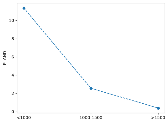
Like in the spatio-temporal analysis, the plots at the landscape level can obtained by not providing any class_val argument.
In order to visualize such information in space, the zonal statistics can be computed in the form of a geo-data frame with the compute_zonal_statistics_gdf method as in:
metrics = ["proportion_of_landscape", "edge_density"]
zonal_statistics_gdf = za.compute_zonal_statistics_gdf(
    metrics=metrics, class_val=URBAN_CLASS_VAL
)

zonal_statistics_gdf.head()
[ ] | 0% Completed | 143.33 us
[########################################] | 100% Completed | 101.12 ms
| edge_density | proportion_of_landscape | geometry | |
|---|---|---|---|
| elev-zone | |||
| 1000-1500 | 6.931125 | 2.550131 | POLYGON ((2563899.597 1160700.222, 2563899.594... |
| <1000 | 27.345710 | 11.364777 | MULTIPOLYGON (((2560899.573 1150500.318, 25606... |
| >1500 | 1.369863 | 0.391389 | MULTIPOLYGON (((2566299.561 1151500.225, 25664... |
the computed metrics are essentially the same as those obtained using the compute_class_metrics_df or compute_landscape_metrics_df (depending on whether a class_val argument is provided or not), with an additional column featuring the vector geometry of each zone. This actually corresponds to a geopandas geo-data frame, and as such, we can use its geopandas.GeoDataFrame.explore method to obtain an interactive map as in:
zonal_statistics_gdf.explore()
Spatio-temporal zonal analysis#
We might also be interested in performing the same zonal analysis at different points in time. This is why pylandstats features an additional SpatioTemporalZonalAnalysis analysis class - as well as SpatioTemporalBufferAnalysis and SpatioTemporalZonalGridAnalysis. See the notebook 04-spatiotemporal-zonal-analysis.ipynb for a more thorough demonstration.
Let us take the sequence of landscapes input_filepaths from the spatio-temporal analysis above and let us use again the dates argument to specify the dates that correspond to each landscape.
Let us also take the latitude and longitude of the center of Lausanne as well as the elevation zones from the zonal analysis above. Now we can construct our SpatioTemporalZonalAnalysis instance and evaluate the sensitive of our spatio-temporal analysis to the extent of the map:
stza = pls.SpatioTemporalZonalAnalysis(
    input_filepaths, elev_zones_filepath, dates=years, zone_index="elev-zone"
)
stza.compute_class_metrics_df()
[ ] | 0% Completed | 137.50 us
[ ] | 0% Completed | 122.56 ms
[ ] | 0% Completed | 237.45 ms
[ ] | 0% Completed | 339.15 ms
[### ] | 8% Completed | 441.20 ms
[### ] | 8% Completed | 558.09 ms
/home/docs/checkouts/readthedocs.org/user_builds/pylandstats/checkouts/latest/.pixi/envs/doc/lib/python3.14/site-packages/numpy/_core/fromnumeric.py:3862: RuntimeWarning: Mean of empty slice
  return _methods._mean(a, axis=axis, dtype=dtype,
/home/docs/checkouts/readthedocs.org/user_builds/pylandstats/checkouts/latest/.pixi/envs/doc/lib/python3.14/site-packages/numpy/_core/_methods.py:142: RuntimeWarning: invalid value encountered in scalar divide
  ret = ret.dtype.type(ret / rcount)
/home/docs/checkouts/readthedocs.org/user_builds/pylandstats/checkouts/latest/src/pylandstats/landscape.py:737: SmallSampleWarning: One or more sample arguments is too small; all returned values will be NaN. See documentation for sample size requirements.
  return reduce_method(patch_metrics)
[### ] | 8% Completed | 671.08 ms
[### ] | 8% Completed | 772.19 ms
[###### ] | 16% Completed | 889.63 ms
[###### ] | 16% Completed | 1.01 s
[############# ] | 33% Completed | 1.11 s
[############# ] | 33% Completed | 1.24 s
/home/docs/checkouts/readthedocs.org/user_builds/pylandstats/checkouts/latest/.pixi/envs/doc/lib/python3.14/site-packages/numpy/_core/fromnumeric.py:3862: RuntimeWarning: Mean of empty slice
  return _methods._mean(a, axis=axis, dtype=dtype,
/home/docs/checkouts/readthedocs.org/user_builds/pylandstats/checkouts/latest/.pixi/envs/doc/lib/python3.14/site-packages/numpy/_core/_methods.py:142: RuntimeWarning: invalid value encountered in scalar divide
  ret = ret.dtype.type(ret / rcount)
/home/docs/checkouts/readthedocs.org/user_builds/pylandstats/checkouts/latest/src/pylandstats/landscape.py:737: SmallSampleWarning: One or more sample arguments is too small; all returned values will be NaN. See documentation for sample size requirements.
  return reduce_method(patch_metrics)
[############# ] | 33% Completed | 1.36 s
[############# ] | 33% Completed | 1.46 s
[############# ] | 33% Completed | 1.56 s
[############# ] | 33% Completed | 1.66 s
[############# ] | 33% Completed | 1.77 s
[#################### ] | 50% Completed | 1.87 s
[#################### ] | 50% Completed | 2.04 s
[#################### ] | 50% Completed | 2.14 s
[#################### ] | 50% Completed | 2.25 s
[########################## ] | 66% Completed | 2.35 s
/home/docs/checkouts/readthedocs.org/user_builds/pylandstats/checkouts/latest/.pixi/envs/doc/lib/python3.14/site-packages/numpy/_core/fromnumeric.py:3862: RuntimeWarning: Mean of empty slice
  return _methods._mean(a, axis=axis, dtype=dtype,
/home/docs/checkouts/readthedocs.org/user_builds/pylandstats/checkouts/latest/.pixi/envs/doc/lib/python3.14/site-packages/numpy/_core/_methods.py:142: RuntimeWarning: invalid value encountered in scalar divide
  ret = ret.dtype.type(ret / rcount)
/home/docs/checkouts/readthedocs.org/user_builds/pylandstats/checkouts/latest/src/pylandstats/landscape.py:737: SmallSampleWarning: One or more sample arguments is too small; all returned values will be NaN. See documentation for sample size requirements.
  return reduce_method(patch_metrics)
/home/docs/checkouts/readthedocs.org/user_builds/pylandstats/checkouts/latest/src/pylandstats/landscape.py:737: SmallSampleWarning: One or more sample arguments is too small; all returned values will be NaN. See documentation for sample size requirements.
  return reduce_method(patch_metrics)
[########################## ] | 66% Completed | 2.50 s
[########################## ] | 66% Completed | 2.60 s
[############################## ] | 75% Completed | 2.71 s
[############################## ] | 75% Completed | 2.83 s
/home/docs/checkouts/readthedocs.org/user_builds/pylandstats/checkouts/latest/.pixi/envs/doc/lib/python3.14/site-packages/numpy/_core/fromnumeric.py:3862: RuntimeWarning: Mean of empty slice
  return _methods._mean(a, axis=axis, dtype=dtype,
/home/docs/checkouts/readthedocs.org/user_builds/pylandstats/checkouts/latest/.pixi/envs/doc/lib/python3.14/site-packages/numpy/_core/_methods.py:142: RuntimeWarning: invalid value encountered in scalar divide
  ret = ret.dtype.type(ret / rcount)
/home/docs/checkouts/readthedocs.org/user_builds/pylandstats/checkouts/latest/src/pylandstats/landscape.py:737: SmallSampleWarning: One or more sample arguments is too small; all returned values will be NaN. See documentation for sample size requirements.
  return reduce_method(patch_metrics)
[################################# ] | 83% Completed | 2.94 s
[################################# ] | 83% Completed | 3.06 s
/home/docs/checkouts/readthedocs.org/user_builds/pylandstats/checkouts/latest/.pixi/envs/doc/lib/python3.14/site-packages/numpy/_core/fromnumeric.py:3862: RuntimeWarning: Mean of empty slice
  return _methods._mean(a, axis=axis, dtype=dtype,
/home/docs/checkouts/readthedocs.org/user_builds/pylandstats/checkouts/latest/.pixi/envs/doc/lib/python3.14/site-packages/numpy/_core/_methods.py:142: RuntimeWarning: invalid value encountered in scalar divide
  ret = ret.dtype.type(ret / rcount)
/home/docs/checkouts/readthedocs.org/user_builds/pylandstats/checkouts/latest/src/pylandstats/landscape.py:737: SmallSampleWarning: One or more sample arguments is too small; all returned values will be NaN. See documentation for sample size requirements.
  return reduce_method(patch_metrics)
[########################################] | 100% Completed | 3.17 s
/home/docs/checkouts/readthedocs.org/user_builds/pylandstats/checkouts/latest/.pixi/envs/doc/lib/python3.14/site-packages/numpy/_core/fromnumeric.py:3862: RuntimeWarning: Mean of empty slice
  return _methods._mean(a, axis=axis, dtype=dtype,
/home/docs/checkouts/readthedocs.org/user_builds/pylandstats/checkouts/latest/.pixi/envs/doc/lib/python3.14/site-packages/numpy/_core/_methods.py:142: RuntimeWarning: invalid value encountered in scalar divide
  ret = ret.dtype.type(ret / rcount)
/home/docs/checkouts/readthedocs.org/user_builds/pylandstats/checkouts/latest/src/pylandstats/landscape.py:1285: RuntimeWarning: Class 1 has less than 2 patches. Euclidean-nearest-neighbor might contain nan values
  warnings.warn(
/home/docs/checkouts/readthedocs.org/user_builds/pylandstats/checkouts/latest/.pixi/envs/doc/lib/python3.14/site-packages/numpy/_core/fromnumeric.py:3862: RuntimeWarning: Mean of empty slice
  return _methods._mean(a, axis=axis, dtype=dtype,
/home/docs/checkouts/readthedocs.org/user_builds/pylandstats/checkouts/latest/.pixi/envs/doc/lib/python3.14/site-packages/numpy/_core/_methods.py:142: RuntimeWarning: invalid value encountered in scalar divide
  ret = ret.dtype.type(ret / rcount)
/home/docs/checkouts/readthedocs.org/user_builds/pylandstats/checkouts/latest/src/pylandstats/landscape.py:737: SmallSampleWarning: One or more sample arguments is too small; all returned values will be NaN. See documentation for sample size requirements.
  return reduce_method(patch_metrics)
| total_area | proportion_of_landscape | number_of_patches | patch_density | largest_patch_index | total_edge | edge_density | total_core_area | core_area_proportion_of_landscape | number_of_disjunct_core_areas | ... | euclidean_nearest_neighbor_md | euclidean_nearest_neighbor_ra | euclidean_nearest_neighbor_sd | euclidean_nearest_neighbor_cv | disjunct_core_area_mn | disjunct_core_area_am | disjunct_core_area_md | disjunct_core_area_ra | disjunct_core_area_sd | disjunct_core_area_cv | |||
|---|---|---|---|---|---|---|---|---|---|---|---|---|---|---|---|---|---|---|---|---|---|---|---|
| class_val | elev-zone | date | |||||||||||||||||||||
| 1 | <1000 | 1980 | 600.0 | 7.526342 | 253 | 3.173608 | 0.765178 | 175100.0 | 21.964375 | 24.0 | 0.301054 | 8 | ... | 223.606798 | 581.024968 | 120.302601 | 42.233561 | 3.000000 | 5.750000 | 2.0 | 9.0 | 2.872281 | 95.742711 |
| 1992 | 678.0 | 8.504767 | 253 | 3.173608 | 0.978424 | 190200.0 | 23.858505 | 27.0 | 0.338685 | 9 | ... | 223.606798 | 581.024968 | 109.769547 | 39.608538 | 3.000000 | 8.259259 | 1.0 | 13.0 | 3.972125 | 132.404170 | ||
| 2004 | 784.0 | 9.834420 | 252 | 3.161064 | 1.141495 | 204500.0 | 25.652283 | 48.0 | 0.602107 | 10 | ... | 223.606798 | 581.024968 | 107.584825 | 39.364455 | 4.800000 | 11.125000 | 2.5 | 16.0 | 5.509991 | 114.791478 | ||
| 2013 | 906.0 | 11.364777 | 235 | 2.947817 | 2.270447 | 218000.0 | 27.345710 | 87.0 | 1.091320 | 17 | ... | 223.606798 | 561.577311 | 104.264469 | 38.169258 | 5.117647 | 21.068966 | 1.0 | 31.0 | 9.035110 | 176.548132 | ||
| 1000-1500 | 1980 | 88.0 | 1.918047 | 44 | 0.959024 | 0.370532 | 27700.0 | 6.037489 | 1.0 | 0.021796 | 1 | ... | 300.000000 | 2616.025568 | 523.560381 | 106.374254 | 1.000000 | 1.000000 | 1.0 | 0.0 | 0.000000 | 0.000000 | |
| 1992 | 101.0 | 2.201395 | 49 | 1.068003 | 0.370532 | 30900.0 | 6.734961 | 1.0 | 0.021796 | 1 | ... | 300.000000 | 2216.609195 | 353.112384 | 89.133340 | 1.000000 | 1.000000 | 1.0 | 0.0 | 0.000000 | 0.000000 | ||
| 2004 | 108.0 | 2.353967 | 46 | 1.002616 | 0.414124 | 30600.0 | 6.669573 | 2.0 | 0.043592 | 2 | ... | 316.227766 | 2216.609195 | 445.954472 | 95.305367 | 1.000000 | 1.000000 | 1.0 | 0.0 | 0.000000 | 0.000000 | ||
| 2013 | 117.0 | 2.550131 | 48 | 1.046207 | 0.457716 | 31800.0 | 6.931125 | 2.0 | 0.043592 | 2 | ... | 360.555128 | 2216.609195 | 439.448544 | 90.250243 | 1.000000 | 1.000000 | 1.0 | 0.0 | 0.000000 | 0.000000 | ||
| >1500 | 1980 | 1.0 | 0.195695 | 1 | 0.195695 | 0.195695 | 300.0 | 0.587084 | 0.0 | 0.000000 | 0 | ... | NaN | NaN | NaN | NaN | NaN | NaN | NaN | NaN | NaN | NaN | |
| 1992 | 2.0 | 0.391389 | 2 | 0.391389 | 0.195695 | 700.0 | 1.369863 | 0.0 | 0.000000 | 0 | ... | 921.954446 | 0.000000 | 0.000000 | 0.000000 | NaN | NaN | NaN | NaN | NaN | NaN | ||
| 2004 | 2.0 | 0.391389 | 2 | 0.391389 | 0.195695 | 700.0 | 1.369863 | 0.0 | 0.000000 | 0 | ... | 921.954446 | 0.000000 | 0.000000 | 0.000000 | NaN | NaN | NaN | NaN | NaN | NaN | ||
| 2013 | 2.0 | 0.391389 | 2 | 0.391389 | 0.195695 | 700.0 | 1.369863 | 0.0 | 0.000000 | 0 | ... | 921.954446 | 0.000000 | 0.000000 | 0.000000 | NaN | NaN | NaN | NaN | NaN | NaN | ||
| 2 | <1000 | 1980 | 5977.0 | 74.974912 | 22 | 0.275966 | 72.190166 | 380100.0 | 47.679378 | 3093.0 | 38.798294 | 55 | ... | 223.606798 | 247.213595 | 68.015646 | 27.785957 | 56.236364 | 907.153896 | 2.0 | 1311.0 | 218.752161 | 388.987030 |
| 1992 | 5898.0 | 73.983944 | 23 | 0.288510 | 71.299548 | 390500.0 | 48.983944 | 2967.0 | 37.217762 | 60 | ... | 223.606798 | 247.213595 | 68.679396 | 28.227968 | 49.450000 | 928.797101 | 2.0 | 1406.0 | 208.527490 | 421.693610 | ||
| 2004 | 5788.0 | 72.604114 | 24 | 0.301054 | 70.045158 | 402800.0 | 50.526844 | 2821.0 | 35.386352 | 64 | ... | 211.803399 | 247.213595 | 67.787892 | 28.069708 | 44.078125 | 1471.332506 | 2.0 | 2014.0 | 250.820049 | 569.035205 | ||
| 2013 | 5669.0 | 71.111390 | 27 | 0.338685 | 68.702960 | 412400.0 | 51.731059 | 2698.0 | 33.843452 | 69 | ... | 200.000000 | 247.213595 | 65.228109 | 27.535485 | 39.101449 | 940.644181 | 2.0 | 1522.0 | 187.754167 | 480.171889 | ||
| 1000-1500 | 1980 | 1925.0 | 41.957280 | 33 | 0.719268 | 16.390584 | 189500.0 | 41.303400 | 670.0 | 14.603313 | 48 | ... | 200.000000 | 470.820393 | 85.441505 | 36.094966 | 13.958333 | 70.420896 | 3.0 | 184.0 | 28.073533 | 201.123820 | |
| 1992 | 1845.0 | 40.213601 | 42 | 0.915432 | 12.881430 | 185600.0 | 40.453357 | 636.0 | 13.862249 | 51 | ... | 200.000000 | 561.577311 | 90.565558 | 38.488281 | 12.470588 | 49.616352 | 4.0 | 132.0 | 21.522768 | 172.588231 | ||
| 2004 | 1825.0 | 39.777681 | 42 | 0.915432 | 12.750654 | 182300.0 | 39.734089 | 629.0 | 13.709677 | 55 | ... | 200.000000 | 561.577311 | 88.567736 | 37.925480 | 11.436364 | 47.791733 | 3.0 | 130.0 | 20.390518 | 178.295467 | ||
| 2013 | 1808.0 | 39.407149 | 47 | 1.024412 | 12.532694 | 181400.0 | 39.537925 | 620.0 | 13.513514 | 54 | ... | 200.000000 | 561.577311 | 84.360148 | 36.684093 | 11.481481 | 47.277419 | 3.5 | 128.0 | 20.272898 | 176.570403 | ||
| >1500 | 1980 | 282.0 | 55.185910 | 15 | 2.935421 | 20.156556 | 19300.0 | 37.769080 | 72.0 | 14.090020 | 8 | ... | 223.606798 | 300.000000 | 80.790623 | 30.950050 | 9.000000 | 30.416667 | 4.0 | 44.0 | 13.883443 | 154.260482 | |
| 1992 | 276.0 | 54.011742 | 16 | 3.131115 | 20.156556 | 19400.0 | 37.964775 | 68.0 | 13.307241 | 6 | ... | 200.000000 | 300.000000 | 80.462794 | 31.924216 | 11.333333 | 31.882353 | 6.0 | 44.0 | 15.260698 | 134.653213 | ||
| 2004 | 272.0 | 53.228963 | 17 | 3.326810 | 19.960861 | 19600.0 | 38.356164 | 65.0 | 12.720157 | 5 | ... | 200.000000 | 300.000000 | 79.015018 | 31.735263 | 13.000000 | 33.061538 | 7.0 | 44.0 | 16.149303 | 124.225411 | ||
| 2013 | 267.0 | 52.250489 | 18 | 3.522505 | 19.765166 | 19700.0 | 38.551859 | 61.0 | 11.937378 | 5 | ... | 200.000000 | 300.000000 | 77.136179 | 32.045939 | 12.200000 | 29.590164 | 7.0 | 40.0 | 14.565713 | 119.391092 | ||
| 3 | <1000 | 1980 | 1257.0 | 15.767687 | 150 | 1.881586 | 2.483693 | 205600.0 | 25.790266 | 189.0 | 2.370798 | 33 | ... | 223.606798 | 408.276253 | 93.036949 | 34.260346 | 5.727273 | 21.783069 | 3.0 | 55.0 | 9.589365 | 167.433359 |
| 1992 | 1270.0 | 15.930758 | 148 | 1.856498 | 2.483693 | 206000.0 | 25.840442 | 193.0 | 2.420973 | 33 | ... | 223.606798 | 408.276253 | 91.974433 | 33.940847 | 5.848485 | 21.455959 | 3.0 | 55.0 | 9.554061 | 163.359585 | ||
| 2004 | 1279.0 | 16.043653 | 147 | 1.843954 | 2.483693 | 204800.0 | 25.689915 | 202.0 | 2.533869 | 32 | ... | 223.606798 | 528.010989 | 96.075762 | 35.555741 | 6.312500 | 22.158416 | 3.0 | 55.0 | 10.001367 | 158.437499 | ||
| 2013 | 1279.0 | 16.043653 | 148 | 1.856498 | 2.483693 | 205500.0 | 25.777722 | 201.0 | 2.521325 | 32 | ... | 223.606798 | 528.010989 | 96.306488 | 35.249921 | 6.281250 | 22.184080 | 3.0 | 55.0 | 9.994481 | 159.116114 | ||
| 1000-1500 | 1980 | 2493.0 | 54.337402 | 46 | 1.002616 | 39.123801 | 196800.0 | 42.894507 | 1182.0 | 25.762860 | 42 | ... | 200.000000 | 247.213595 | 49.069948 | 21.353026 | 28.142857 | 198.578680 | 5.5 | 345.0 | 69.257137 | 246.091350 | |
| 1992 | 2579.0 | 56.211857 | 39 | 0.850044 | 46.011334 | 196900.0 | 42.916303 | 1247.0 | 27.179599 | 40 | ... | 200.000000 | 247.213595 | 60.406085 | 25.161961 | 31.175000 | 217.995990 | 5.0 | 370.0 | 76.316082 | 244.798980 | ||
| 2004 | 2599.0 | 56.647777 | 41 | 0.893636 | 51.285963 | 192600.0 | 41.979076 | 1285.0 | 28.007847 | 40 | ... | 223.606798 | 247.213595 | 54.298559 | 22.636296 | 32.125000 | 223.272374 | 4.0 | 379.0 | 78.362040 | 243.928530 | ||
| 2013 | 2605.0 | 56.778553 | 41 | 0.893636 | 51.351351 | 192200.0 | 41.891892 | 1287.0 | 28.051439 | 40 | ... | 223.606798 | 247.213595 | 53.922797 | 22.615863 | 32.175000 | 223.891997 | 4.0 | 379.0 | 78.539763 | 244.101828 | ||
| >1500 | 1980 | 97.0 | 18.982387 | 13 | 2.544031 | 8.610568 | 12200.0 | 23.874755 | 9.0 | 1.761252 | 3 | ... | 223.606798 | 384.669455 | 133.129559 | 43.464871 | 3.000000 | 3.888889 | 3.0 | 4.0 | 1.632993 | 54.433105 | |
| 1992 | 102.0 | 19.960861 | 13 | 2.544031 | 8.610568 | 13000.0 | 25.440313 | 9.0 | 1.761252 | 3 | ... | 223.606798 | 384.669455 | 133.129559 | 43.464871 | 3.000000 | 3.888889 | 3.0 | 4.0 | 1.632993 | 54.433105 | ||
| 2004 | 112.0 | 21.917808 | 13 | 2.544031 | 8.806262 | 13300.0 | 26.027397 | 11.0 | 2.152642 | 3 | ... | 300.000000 | 984.697800 | 272.115303 | 71.227231 | 3.666667 | 4.636364 | 5.0 | 4.0 | 1.885618 | 51.425948 | ||
| 2013 | 115.0 | 22.504892 | 13 | 2.544031 | 8.806262 | 13200.0 | 25.831703 | 11.0 | 2.152642 | 3 | ... | 300.000000 | 984.697800 | 271.071081 | 71.191170 | 3.666667 | 4.636364 | 5.0 | 4.0 | 1.885618 | 51.425948 | ||
| 4 | <1000 | 1980 | 138.0 | 1.731059 | 85 | 1.066232 | 0.250878 | 43600.0 | 5.469142 | 3.0 | 0.037632 | 2 | ... | 424.264069 | 1526.267650 | 263.112174 | 56.977578 | 1.500000 | 1.666667 | 1.5 | 1.0 | 0.500000 | 33.333333 |
| 1992 | 126.0 | 1.580532 | 81 | 1.016056 | 0.263422 | 39900.0 | 5.005018 | 3.0 | 0.037632 | 2 | ... | 447.213595 | 1526.267650 | 270.417030 | 55.838766 | 1.500000 | 1.666667 | 1.5 | 1.0 | 0.500000 | 33.333333 | ||
| 2004 | 121.0 | 1.517812 | 80 | 1.003512 | 0.288510 | 37700.0 | 4.729052 | 4.0 | 0.050176 | 2 | ... | 447.213595 | 1214.213562 | 284.662627 | 53.811346 | 2.000000 | 2.000000 | 2.0 | 0.0 | 0.000000 | 0.000000 | ||
| 2013 | 118.0 | 1.480181 | 77 | 0.965881 | 0.288510 | 36700.0 | 4.603613 | 4.0 | 0.050176 | 2 | ... | 447.213595 | 1624.828759 | 295.145638 | 55.658069 | 2.000000 | 2.000000 | 2.0 | 0.0 | 0.000000 | 0.000000 | ||
| 1000-1500 | 1980 | 82.0 | 1.787271 | 58 | 1.264167 | 0.239756 | 28200.0 | 6.146469 | 0.0 | 0.000000 | 0 | ... | 338.391447 | 1160.147051 | 285.154750 | 64.592449 | NaN | NaN | NaN | NaN | NaN | NaN | |
| 1992 | 63.0 | 1.373147 | 50 | 1.089799 | 0.087184 | 23000.0 | 5.013078 | 0.0 | 0.000000 | 0 | ... | 406.155281 | 1440.121947 | 286.874109 | 63.655059 | NaN | NaN | NaN | NaN | NaN | NaN | ||
| 2004 | 56.0 | 1.220575 | 41 | 0.893636 | 0.065388 | 19100.0 | 4.163034 | 0.0 | 0.000000 | 0 | ... | 400.000000 | 1440.121947 | 309.462998 | 63.644295 | NaN | NaN | NaN | NaN | NaN | NaN | ||
| 2013 | 58.0 | 1.264167 | 40 | 0.871840 | 0.065388 | 20400.0 | 4.446382 | 0.0 | 0.000000 | 0 | ... | 406.155281 | 1440.121947 | 357.168210 | 68.905585 | NaN | NaN | NaN | NaN | NaN | NaN | ||
| >1500 | 1980 | 131.0 | 25.636008 | 8 | 1.565558 | 10.371820 | 14200.0 | 27.788650 | 23.0 | 4.500978 | 2 | ... | 300.000000 | 286.295154 | 83.535518 | 27.389163 | 11.500000 | 16.391304 | 11.5 | 15.0 | 7.500000 | 65.217391 | |
| 1992 | 131.0 | 25.636008 | 9 | 1.761252 | 10.763209 | 14100.0 | 27.592955 | 24.0 | 4.696673 | 3 | ... | 282.842712 | 100.000000 | 43.153130 | 16.668188 | 8.000000 | 15.750000 | 4.0 | 18.0 | 7.874008 | 98.425098 | ||
| 2004 | 125.0 | 24.461840 | 11 | 2.152642 | 10.371820 | 13200.0 | 25.831703 | 26.0 | 5.088063 | 3 | ... | 282.842712 | 100.000000 | 45.440807 | 17.920276 | 8.666667 | 17.615385 | 4.0 | 20.0 | 8.806563 | 101.614191 | ||
| 2013 | 127.0 | 24.853229 | 12 | 2.348337 | 10.567515 | 13800.0 | 27.005871 | 26.0 | 5.088063 | 3 | ... | 282.842712 | 200.000000 | 59.419362 | 22.357071 | 8.666667 | 17.615385 | 4.0 | 20.0 | 8.806563 | 101.614191 |
48 rows × 66 columns
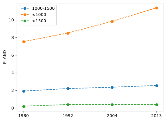
stza.plot_metric("proportion_of_landscape", class_val=URBAN_CLASS_VAL)
[ ] | 0% Completed | 141.34 us
[########################################] | 100% Completed | 101.09 ms
<Axes: ylabel='PLAND'>