Zonal Analysis#
import contextily as cx
import geopandas as gpd
import matplotlib.pyplot as plt
import numpy as np
import rasterio as rio
import swisslandstats as sls
from shapely.geometry import Point

import pylandstats as pls
Landscapes tend to be heterogeneous and complex and therefore reducing such information to a single scalar value for all the landscape often leads to metric values that are hard to interpret. It might thus be helpful to decompose the landscape into a set of zones of interest and compute the metrics for each zone separately. Such approach to GIS is often referred to as zonal analysis. The pylandstats library features three classes that might be used to that end: the more generic ZonalAnalysis, BufferAnalysis and ZonalGridAnalysis.
The data used in this notebook ships with the docs in the data directory, namely:
the land use/land cover (LULC) data is downloaded and preprocessed (see A03-swisslandstats-preprocessing.ipynb for more details).
the elevation zones vector data is downloaded and preprocessed (see A04-elevation-zones.ipynb for more details).
Consider the following landscape of the District of the Veveyse, Switzerland:
URBAN_CLASS_VAL = 1
input_filepath = "data/veveyse/AS18_4.tif"

with rio.open(input_filepath) as src:
    plt.imshow(src.read(1), cmap=sls.noas04_4_cmap, norm=sls.noas04_4_norm)

Zonal analysis#
The ZonalAnalysis class of PyLandStats serves to compute the landscape metrics over any set of zones. Instantiating a ZonalAnalysis requires two positional arguments, namely the landscape file and the zones, which can be defined by means of vector geometries or a labelled array of the same form as the landscape (i.e., mapping each landscape pixel to its zone).
Using vector geometries to define zones#
The most straight-forward way to define a zonal analysis is to use a geopandas geo-series or geo-data frame or its equivalent file-like object. In this example, we will use a geopackage file defining a set of elevation zones. Additionally, we will use the zone_index argument to indicate which column of the geopackage file will be used to index the zones:
elev_zones_filepath = "data/elev-zones.gpkg"

za = pls.ZonalAnalysis(input_filepath, elev_zones_filepath, zone_index="elev-zone")
The ZonalAnalysis instance will automatically generate the three landscapes of interest (one for each transect) by masking the pixels of the input raster. Such information is stored as part of the zone_gser attribute:
za.zone_gser
elev-zone
<1000        MULTIPOLYGON (((2560899.573 1150500.318, 25606...
1000-1500    POLYGON ((2563899.597 1160700.222, 2563899.594...
>1500        MULTIPOLYGON (((2566299.561 1151500.225, 25664...
Name: geometry, dtype: geometry
We can also plot the zone_gser attribute to visualize the zones (we are resetting the index so that we can use it as color scheme) with a basemap (obtained using the contextily library):
ax = za.zone_gser.reset_index().plot(
    "elev-zone", alpha=0.6, categorical=True, legend=True
)
cx.add_basemap(ax, crs=za.zone_gser.crs, source=cx.providers.CartoDB.Positron)

Similarly, we can visualize the landscape rasters of each zone by means of the plot_landscapes method as in:
fig = za.plot_landscapes(
    cmap=sls.noas04_4_cmap, show_kwargs=dict(norm=sls.noas04_4_norm)
)

The goal is now to compute and plot the landscape metrics for each zone. Like SpatioTemporalAnalysis, ZonalAnalysis only supports class and landscape-level metrics, which again, can be computed by means of its methods compute_class_metrics_df and compute_landscape_metrics_df respectively, e.g.:
za.compute_class_metrics_df()
[ ] | 0% Completed | 195.52 us
[ ] | 0% Completed | 108.57 ms
[ ] | 0% Completed | 266.47 ms
[ ] | 0% Completed | 370.61 ms
[############# ] | 33% Completed | 478.83 ms
[############# ] | 33% Completed | 583.12 ms
/home/docs/checkouts/readthedocs.org/user_builds/pylandstats/checkouts/latest/.pixi/envs/doc/lib/python3.14/site-packages/numpy/_core/fromnumeric.py:3862: RuntimeWarning: Mean of empty slice
  return _methods._mean(a, axis=axis, dtype=dtype,
/home/docs/checkouts/readthedocs.org/user_builds/pylandstats/checkouts/latest/.pixi/envs/doc/lib/python3.14/site-packages/numpy/_core/_methods.py:142: RuntimeWarning: invalid value encountered in scalar divide
  ret = ret.dtype.type(ret / rcount)
/home/docs/checkouts/readthedocs.org/user_builds/pylandstats/checkouts/latest/src/pylandstats/landscape.py:776: SmallSampleWarning: One or more sample arguments is too small; all returned values will be NaN. See documentation for sample size requirements.
  return reduce_method(patch_metrics)
[########################################] | 100% Completed | 685.41 ms
/home/docs/checkouts/readthedocs.org/user_builds/pylandstats/checkouts/latest/.pixi/envs/doc/lib/python3.14/site-packages/numpy/_core/fromnumeric.py:3862: RuntimeWarning: Mean of empty slice
  return _methods._mean(a, axis=axis, dtype=dtype,
/home/docs/checkouts/readthedocs.org/user_builds/pylandstats/checkouts/latest/.pixi/envs/doc/lib/python3.14/site-packages/numpy/_core/_methods.py:142: RuntimeWarning: invalid value encountered in scalar divide
  ret = ret.dtype.type(ret / rcount)
/home/docs/checkouts/readthedocs.org/user_builds/pylandstats/checkouts/latest/src/pylandstats/landscape.py:776: SmallSampleWarning: One or more sample arguments is too small; all returned values will be NaN. See documentation for sample size requirements.
  return reduce_method(patch_metrics)
| total_area | proportion_of_landscape | number_of_patches | patch_density | largest_patch_index | total_edge | edge_density | total_core_area | core_area_proportion_of_landscape | number_of_disjunct_core_areas | ... | euclidean_nearest_neighbor_md | euclidean_nearest_neighbor_ra | euclidean_nearest_neighbor_sd | euclidean_nearest_neighbor_cv | disjunct_core_area_mn | disjunct_core_area_am | disjunct_core_area_md | disjunct_core_area_ra | disjunct_core_area_sd | disjunct_core_area_cv | ||
|---|---|---|---|---|---|---|---|---|---|---|---|---|---|---|---|---|---|---|---|---|---|---|
| class_val | elev-zone | |||||||||||||||||||||
| 1 | <1000 | 906.0 | 11.364777 | 235 | 2.947817 | 2.270447 | 218000.0 | 27.345710 | 87.0 | 1.091320 | 17 | ... | 223.606798 | 561.577311 | 104.264469 | 38.169258 | 5.117647 | 21.068966 | 1.0 | 31.0 | 9.035110 | 176.548132 |
| 1000-1500 | 117.0 | 2.550131 | 48 | 1.046207 | 0.457716 | 31800.0 | 6.931125 | 2.0 | 0.043592 | 2 | ... | 360.555128 | 2216.609195 | 439.448544 | 90.250243 | 1.000000 | 1.000000 | 1.0 | 0.0 | 0.000000 | 0.000000 | |
| >1500 | 2.0 | 0.391389 | 2 | 0.391389 | 0.195695 | 700.0 | 1.369863 | 0.0 | 0.000000 | 0 | ... | 921.954446 | 0.000000 | 0.000000 | 0.000000 | NaN | NaN | NaN | NaN | NaN | NaN | |
| 2 | <1000 | 5543.0 | 69.530858 | 30 | 0.376317 | 67.222780 | 434400.0 | 54.490718 | 2482.0 | 31.133969 | 82 | ... | 200.000000 | 247.213595 | 62.304711 | 26.538335 | 30.268293 | 489.738920 | 3.0 | 984.0 | 117.929604 | 389.614323 |
| 1000-1500 | 1611.0 | 35.113339 | 57 | 1.242371 | 10.200523 | 196400.0 | 42.807323 | 436.0 | 9.503051 | 60 | ... | 200.000000 | 624.621125 | 88.650569 | 38.186111 | 7.266667 | 29.729358 | 2.5 | 85.0 | 12.776106 | 175.817975 | |
| >1500 | 247.0 | 48.336595 | 19 | 3.718200 | 18.590998 | 21200.0 | 41.487280 | 49.0 | 9.589041 | 7 | ... | 200.000000 | 300.000000 | 82.560212 | 32.574672 | 7.000000 | 17.122449 | 5.0 | 26.0 | 8.417668 | 120.252407 | |
| 3 | <1000 | 1464.0 | 18.364275 | 225 | 2.822378 | 2.558956 | 257200.0 | 32.262920 | 208.0 | 2.609132 | 36 | ... | 223.606798 | 521.110255 | 82.910720 | 31.969439 | 5.777778 | 21.548077 | 2.5 | 55.0 | 9.545537 | 165.211224 |
| 1000-1500 | 2815.0 | 61.355711 | 39 | 0.850044 | 56.952921 | 211700.0 | 46.142110 | 1377.0 | 30.013078 | 44 | ... | 223.606798 | 116.227766 | 38.872836 | 16.909566 | 31.295455 | 243.698620 | 4.0 | 425.0 | 81.530691 | 260.519275 | |
| >1500 | 143.0 | 27.984344 | 19 | 3.718200 | 9.001957 | 17500.0 | 34.246575 | 13.0 | 2.544031 | 4 | ... | 223.606798 | 383.095189 | 108.334494 | 38.595026 | 3.250000 | 4.230769 | 3.5 | 4.0 | 1.785357 | 54.934065 | |
| 4 | <1000 | 59.0 | 0.740090 | 25 | 0.313598 | 0.288510 | 14600.0 | 1.831410 | 4.0 | 0.050176 | 2 | ... | 447.213595 | 2117.333184 | 553.411820 | 79.274675 | 2.000000 | 2.000000 | 2.0 | 0.0 | 0.000000 | 0.000000 |
| 1000-1500 | 45.0 | 0.980820 | 33 | 0.719268 | 0.065388 | 16100.0 | 3.509154 | 0.0 | 0.000000 | 0 | ... | 360.555128 | 1440.121947 | 414.967474 | 76.470603 | NaN | NaN | NaN | NaN | NaN | NaN | |
| >1500 | 119.0 | 23.287671 | 11 | 2.152642 | 9.784736 | 14000.0 | 27.397260 | 23.0 | 4.500978 | 3 | ... | 282.842712 | 247.213595 | 80.782967 | 29.264315 | 7.666667 | 14.826087 | 4.0 | 17.0 | 7.408704 | 96.635264 |
12 rows × 66 columns
Likewise SpatioTemporalAnalysis, if we want to compute the metrics data frame only for a subset of metrics or classes, or customize how the metrics are computed, we must pass the arguments metrics, classes or metrics_kwargs to the compute_class_metrics_df and compute_landscape_metrics_df, as in:
metrics = ["proportion_of_landscape", "edge_density", "fractal_dimension_am"]
classes = [URBAN_CLASS_VAL]
metrics_kwargs = {
    "proportion_of_landscape": {"percent": False},
    "edge_density": {"count_boundary": True},
}
za.compute_class_metrics_df(
    metrics=metrics, classes=[URBAN_CLASS_VAL], metrics_kwargs=metrics_kwargs
)
[ ] | 0% Completed | 168.84 us
[########################################] | 100% Completed | 101.45 ms
| proportion_of_landscape | edge_density | fractal_dimension_am | ||
|---|---|---|---|---|
| class_val | elev-zone | |||
| 1 | <1000 | 0.113648 | 27.872554 | 1.117441 |
| 1000-1500 | 0.025501 | 7.149085 | 1.068271 | |
| >1500 | 0.003914 | 1.565558 | 1.000000 |
On the other hand, the plot_metric method of ZonalAnalysis will plot the value of a given metric for each zone:
za.plot_metric("proportion_of_landscape", class_val=URBAN_CLASS_VAL)
[ ] | 0% Completed | 130.41 us
[########################################] | 100% Completed | 100.80 ms
<Axes: ylabel='PLAND'>
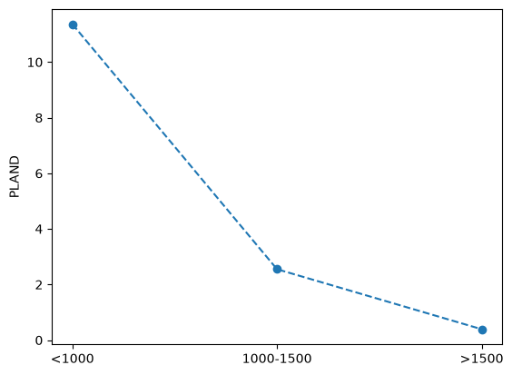
In this case we see how the proportion of urbanized landscape (class 1) becomes zero at highest altitudes.
Finally, in order to visualize such information in space, the zonal statistics can be computed in the form of a geo-data frame with the compute_zonal_statistics_gdf method as in:
zonal_statistics_gdf = za.compute_zonal_statistics_gdf(
    metrics=metrics, class_val=URBAN_CLASS_VAL
)
zonal_statistics_gdf.head()
[ ] | 0% Completed | 152.89 us
[########################################] | 100% Completed | 101.06 ms
| edge_density | fractal_dimension_am | proportion_of_landscape | geometry | |
|---|---|---|---|---|
| elev-zone | ||||
| 1000-1500 | 6.931125 | 1.068271 | 2.550131 | POLYGON ((2563899.597 1160700.222, 2563899.594... |
| <1000 | 27.345710 | 1.117441 | 11.364777 | MULTIPOLYGON (((2560899.573 1150500.318, 25606... |
| >1500 | 1.369863 | 1.000000 | 0.391389 | MULTIPOLYGON (((2566299.561 1151500.225, 25664... |
zonal_statistics_gdf.plot("edge_density")
<Axes: >

The computed metrics are essentially the same as those obtained using the compute_class_metrics_df or compute_landscape_metrics_df (depending on whether a class_val argument is provided or not), with an additional column featuring the vector geometry of each zone. This actually corresponds to a geopandas geo-data frame, and as such, we can use its geopandas.GeoDataFrame.plot method to spatially visualize the value of a metric across the zones:
zonal_statistics_gdf.plot("proportion_of_landscape", legend=True)
<Axes: >

Using labelled raster arrays to define zones#
The zones can be defined as NumPy labelled arrays of the same shape of the landscape of interest, where each zone is labelled by a unique integer value, which will be used to identify the zones (i.e., as index).
For instance, in order to compute the metrics over a set of rectangular transects, let us define three transects of 50x50 cells (5x5km) that horizontally traverse our landscape at the latitude of Chatel-St-Denis:
with rio.open(input_filepath) as src:
    label_arr = np.zeros(src.shape, dtype=np.uint8)

transect_len = 50
for i, transect_start in enumerate(range(0, 150, transect_len), start=1):
    label_arr[80:130, transect_start : transect_start + transect_len] = i

plt.imshow(label_arr)
plt.colorbar()
<matplotlib.colorbar.Colorbar at 0x78fe2a622ba0>
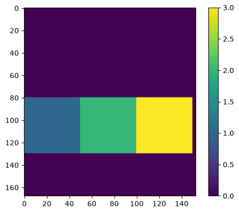
As we can see, the array labels each transect zone by a unique integer. We can use it as the zones argument when initializing a ZonalAnalysis instance:
za = pls.ZonalAnalysis(input_filepath, label_arr)
za.compute_zonal_statistics_gdf(
    metrics=["proportion_of_landscape"], class_val=URBAN_CLASS_VAL
)
[ ] | 0% Completed | 138.84 us
[########################################] | 100% Completed | 101.02 ms
/home/docs/checkouts/readthedocs.org/user_builds/pylandstats/checkouts/latest/.pixi/envs/doc/lib/python3.14/site-packages/pyogrio/raw.py:200: RuntimeWarning: Invalid range specified
  return ogr_read(
| proportion_of_landscape | geometry | |
|---|---|---|
| zone | ||
| 1.0 | 14.167813 | POLYGON ((2551850 1156050, 2551850 1151050, 25... |
| 2.0 | 14.092256 | POLYGON ((2556850 1156050, 2556850 1151050, 25... |
| 3.0 | 3.752182 | POLYGON ((2561850 1156050, 2561850 1151050, 25... |
Note from the geo-data frame above that the label values are used to index the zones. We can override this behaviour by providing a custom zone_index argument, e.g., strings that denote that each landscape corresponds to the transect from kilometers 0 to 5, 5 to 10 and 10 to 15 respectivel:
za = pls.ZonalAnalysis(input_filepath, label_arr, zone_index=["0-5", "5-10", "10-15"])
za.compute_zonal_statistics_gdf(
    metrics=["proportion_of_landscape"], class_val=URBAN_CLASS_VAL
)
[ ] | 0% Completed | 160.65 us
/home/docs/checkouts/readthedocs.org/user_builds/pylandstats/checkouts/latest/.pixi/envs/doc/lib/python3.14/site-packages/pyogrio/raw.py:200: RuntimeWarning: Invalid range specified
  return ogr_read(
[########################################] | 100% Completed | 101.43 ms
| proportion_of_landscape | geometry | |
|---|---|---|
| zone | ||
| 0-5 | 14.167813 | POLYGON ((2551850 1156050, 2551850 1151050, 25... |
| 10-15 | 3.752182 | POLYGON ((2561850 1156050, 2561850 1151050, 25... |
| 5-10 | 14.092256 | POLYGON ((2556850 1156050, 2556850 1151050, 25... |
We can see that the highest proportion of urban land cover is found in the western and central transects, which actually correspond to the town of Chatel-St-Denis.
Buffer Analysis#
In line with the classic concentric models of location and land use, we are often interested in evaluate how the landscape patterns change as we move away from the urban center. This is similar to the “gradient analysis” approach from landscape ecology, which consists in evaluating the spatial variation of the landscape patterns as one moves progressively from the highly-developed urban cores to the less intense suburbs until the rural and natural hinterlands.
To that end, PyLandStats features the BufferAnalysis class (which inherits from the ZonalAnalysis class), which defines a series of spatial extents for our landscape based on buffers of increasing distances around our feature of interest - in this example, the town of Chatel-St-Denis.
From Point#
We might define a given coordinate as the center of our region of interest (in this example, the town of Chatel-St-Denis) and a series of buffer distances around that point:
# latitude and longitude of the center of Chatel-St-Denis according to OpenStreetMap
base_geom = Point(6.8992073, 46.52634)
base_geom_crs = "+proj=longlat +ellps=WGS84 +datum=WGS84 +no_defs"

# buffer distances (in meters)
buffer_dists = [2000, 4000, 6000]
then, we can use the BufferAnalysis class of Pylandstats as in (note that in this case we need to provide the CRS of the geometry using the base_geom_crs):
ba = pls.BufferAnalysis(
    input_filepath, base_geom, buffer_dists, base_geom_crs=base_geom_crs
)
The BufferAnalysis instance will automatically generate the three landscapes of interest (one for each buffer distance) by masking the pixels of the input raster:
fig = ba.plot_landscapes(
    cmap=sls.noas04_4_cmap, show_kwargs=dict(norm=sls.noas04_4_norm)
)

Likewise ZonalAnalysis, we can compute the landscap metrics for each buffer distance with the compute_class_metrics_df and compute_landscape_metrics_df methods, e.g.:
ba.compute_class_metrics_df()
[ ] | 0% Completed | 136.42 us
[ ] | 0% Completed | 104.06 ms
[ ] | 0% Completed | 210.45 ms
[ ] | 0% Completed | 323.45 ms
[ ] | 0% Completed | 426.25 ms
[############# ] | 33% Completed | 547.08 ms
[########################################] | 100% Completed | 652.56 ms
| total_area | proportion_of_landscape | number_of_patches | patch_density | largest_patch_index | total_edge | edge_density | total_core_area | core_area_proportion_of_landscape | number_of_disjunct_core_areas | ... | euclidean_nearest_neighbor_md | euclidean_nearest_neighbor_ra | euclidean_nearest_neighbor_sd | euclidean_nearest_neighbor_cv | disjunct_core_area_mn | disjunct_core_area_am | disjunct_core_area_md | disjunct_core_area_ra | disjunct_core_area_sd | disjunct_core_area_cv | ||
|---|---|---|---|---|---|---|---|---|---|---|---|---|---|---|---|---|---|---|---|---|---|---|
| class_val | buffer_dist | |||||||||||||||||||||
| 1 | 2000 | 281.0 | 24.224138 | 25 | 2.155172 | 16.465517 | 50900.0 | 43.879310 | 45.0 | 3.879310 | 7 | ... | 223.606798 | 365.685425 | 98.258940 | 38.735937 | 6.428571 | 23.755556 | 1.0 | 31.0 | 10.554040 | 164.173952 |
| 4000 | 469.0 | 12.727273 | 75 | 2.035278 | 5.183175 | 97700.0 | 26.512890 | 52.0 | 1.411126 | 13 | ... | 223.606798 | 528.010989 | 119.039983 | 42.131915 | 4.000000 | 20.730769 | 1.0 | 31.0 | 8.180653 | 204.516315 | |
| 6000 | 785.0 | 10.910354 | 158 | 2.195969 | 2.654621 | 170300.0 | 23.669215 | 88.0 | 1.223072 | 18 | ... | 223.606798 | 1100.000000 | 130.265430 | 47.329386 | 4.888889 | 20.840909 | 1.0 | 31.0 | 8.831062 | 180.635357 | |
| 2 | 2000 | 664.0 | 57.241379 | 11 | 0.948276 | 43.793103 | 76000.0 | 65.517241 | 186.0 | 16.034483 | 27 | ... | 200.000000 | 100.000000 | 28.747979 | 13.749033 | 6.888889 | 44.236559 | 2.0 | 79.0 | 16.040073 | 232.839773 |
| 4000 | 2090.0 | 56.716418 | 24 | 0.651289 | 45.210312 | 213100.0 | 57.829037 | 744.0 | 20.189959 | 55 | ... | 200.000000 | 160.555128 | 41.964441 | 19.106554 | 13.527273 | 110.846774 | 2.0 | 239.0 | 36.283156 | 268.222258 | |
| 6000 | 4042.0 | 56.177901 | 42 | 0.583739 | 46.309937 | 394500.0 | 54.829743 | 1515.0 | 21.056289 | 96 | ... | 200.000000 | 100.000000 | 20.917722 | 9.909001 | 15.781250 | 140.441584 | 3.0 | 312.0 | 44.354209 | 281.056377 | |
| 3 | 2000 | 193.0 | 16.637931 | 41 | 3.534483 | 3.965517 | 38700.0 | 33.362069 | 14.0 | 1.206897 | 4 | ... | 200.000000 | 528.010989 | 114.864913 | 43.048566 | 3.500000 | 6.571429 | 2.0 | 8.0 | 3.278719 | 93.677693 |
| 4000 | 1088.0 | 29.525102 | 89 | 2.415197 | 10.719132 | 151300.0 | 41.058345 | 276.0 | 7.489824 | 27 | ... | 200.000000 | 521.110255 | 88.182057 | 36.383994 | 10.222222 | 32.782609 | 3.0 | 58.0 | 15.186089 | 148.559561 | |
| 6000 | 2303.0 | 32.008339 | 143 | 1.987491 | 20.625434 | 293500.0 | 40.792217 | 678.0 | 9.423211 | 53 | ... | 223.606798 | 581.024968 | 99.700945 | 38.087863 | 12.792453 | 92.356932 | 4.0 | 221.0 | 31.903367 | 249.392105 | |
| 4 | 2000 | 22.0 | 1.896552 | 7 | 0.603448 | 1.379310 | 3800.0 | 3.275862 | 2.0 | 0.172414 | 1 | ... | 447.213595 | 934.166406 | 328.138816 | 50.665030 | 2.000000 | 2.000000 | 2.0 | 0.0 | 0.000000 | 0.000000 |
| 4000 | 38.0 | 1.031208 | 11 | 0.298507 | 0.624152 | 7700.0 | 2.089552 | 4.0 | 0.108548 | 2 | ... | 447.213595 | 1296.223784 | 453.723564 | 61.663637 | 2.000000 | 2.000000 | 2.0 | 0.0 | 0.000000 | 0.000000 | |
| 6000 | 65.0 | 0.903405 | 32 | 0.444753 | 0.319666 | 16900.0 | 2.348853 | 4.0 | 0.055594 | 2 | ... | 447.213595 | 1620.302094 | 484.871538 | 67.943934 | 2.000000 | 2.000000 | 2.0 | 0.0 | 0.000000 | 0.000000 |
12 rows × 66 columns
Note that the data frames for BufferAnalysis, likewise those of SpatioTemporalAnalysis or ZonalAnalysis (see above) can be customized via by passing the arguments metrics, classes or metrics_kws to the compute_class_metrics_df and compute_landscape_metrics_df methods.
The plot_metric method of BufferAnalysis will plot the value of a given metric for each of the buffered landscapes:
ba.plot_metric("proportion_of_landscape", class_val=URBAN_CLASS_VAL)
[ ] | 0% Completed | 119.83 us
[########################################] | 100% Completed | 101.69 ms
<Axes: ylabel='PLAND'>

The specific plot above shows how the proportion of landscape (y-axis) occupied by urban land uses diminishes with the buffer distance (x-axis) around the feature of interest (i.e., the city center of Chatel-St-Denis).
To examine more closely how landscape patterns change as we move along the urban-rural gradient, we might actually want to compute the metrics for each of the buffer rings that lie within each pair of increasing buffer distances. For instance, for the buffer distances considered in this example (i.e., 2000, 4000 and 6000), we would like to compute the metrics for the buffer rings that go from 0 to 2000m, 2000 to 4000m and 4000 to 6000m around the center of Chatel-St-Denis).
To that end, we might pass the argument buffer_rings=True when instantiating BufferAnalysis as in:
ba = pls.BufferAnalysis(
    input_filepath,
    base_geom,
    buffer_dists,
    buffer_rings=True,
    base_geom_crs=base_geom_crs,
)
fig = ba.plot_landscapes(
    cmap=sls.noas04_4_cmap, show_kwargs=dict(norm=sls.noas04_4_norm)
)

ba.compute_class_metrics_df()
[ ] | 0% Completed | 187.34 us
[ ] | 0% Completed | 112.51 ms
[ ] | 0% Completed | 241.41 ms
[ ] | 0% Completed | 372.45 ms
[############# ] | 33% Completed | 491.39 ms
[############# ] | 33% Completed | 592.57 ms
[########################################] | 100% Completed | 695.50 ms
/home/docs/checkouts/readthedocs.org/user_builds/pylandstats/checkouts/latest/.pixi/envs/doc/lib/python3.14/site-packages/numpy/_core/fromnumeric.py:3862: RuntimeWarning: Mean of empty slice
  return _methods._mean(a, axis=axis, dtype=dtype,
/home/docs/checkouts/readthedocs.org/user_builds/pylandstats/checkouts/latest/.pixi/envs/doc/lib/python3.14/site-packages/numpy/_core/_methods.py:142: RuntimeWarning: invalid value encountered in scalar divide
  ret = ret.dtype.type(ret / rcount)
/home/docs/checkouts/readthedocs.org/user_builds/pylandstats/checkouts/latest/src/pylandstats/landscape.py:776: SmallSampleWarning: One or more sample arguments is too small; all returned values will be NaN. See documentation for sample size requirements.
  return reduce_method(patch_metrics)
| total_area | proportion_of_landscape | number_of_patches | patch_density | largest_patch_index | total_edge | edge_density | total_core_area | core_area_proportion_of_landscape | number_of_disjunct_core_areas | ... | euclidean_nearest_neighbor_md | euclidean_nearest_neighbor_ra | euclidean_nearest_neighbor_sd | euclidean_nearest_neighbor_cv | disjunct_core_area_mn | disjunct_core_area_am | disjunct_core_area_md | disjunct_core_area_ra | disjunct_core_area_sd | disjunct_core_area_cv | ||
|---|---|---|---|---|---|---|---|---|---|---|---|---|---|---|---|---|---|---|---|---|---|---|
| class_val | buffer_dist | |||||||||||||||||||||
| 1 | 0-2000 | 281.0 | 24.224138 | 25 | 2.155172 | 16.465517 | 50900.0 | 43.879310 | 45.0 | 3.879310 | 7 | ... | 223.606798 | 365.685425 | 98.258940 | 38.735937 | 6.428571 | 23.755556 | 1.0 | 31.0 | 10.554040 | 164.173952 |
| 2000-4000 | 188.0 | 7.445545 | 52 | 2.059406 | 1.544554 | 45600.0 | 18.059406 | 7.0 | 0.277228 | 6 | ... | 223.606798 | 528.010989 | 137.026942 | 45.084053 | 1.166667 | 1.285714 | 1.0 | 1.0 | 0.372678 | 31.943828 | |
| 4000-6000 | 316.0 | 9.002849 | 93 | 2.649573 | 1.794872 | 70500.0 | 20.085470 | 30.0 | 0.854701 | 6 | ... | 223.606798 | 1100.000000 | 133.081707 | 49.608104 | 5.000000 | 14.266667 | 2.0 | 19.0 | 6.806859 | 136.137186 | |
| 2 | 0-2000 | 664.0 | 57.241379 | 11 | 0.948276 | 43.793103 | 76000.0 | 65.517241 | 186.0 | 16.034483 | 27 | ... | 200.000000 | 100.000000 | 28.747979 | 13.749033 | 6.888889 | 44.236559 | 2.0 | 79.0 | 16.040073 | 232.839773 |
| 2000-4000 | 1426.0 | 56.475248 | 19 | 0.752475 | 45.584158 | 132400.0 | 52.435644 | 521.0 | 20.633663 | 36 | ... | 200.000000 | 160.555128 | 45.414311 | 20.091006 | 14.472222 | 90.024952 | 2.0 | 180.0 | 33.066840 | 228.484882 | |
| 4000-6000 | 1952.0 | 55.612536 | 31 | 0.883191 | 28.888889 | 176400.0 | 50.256410 | 729.0 | 20.769231 | 45 | ... | 200.000000 | 200.000000 | 49.255127 | 21.993592 | 16.200000 | 137.463649 | 3.0 | 263.0 | 44.322355 | 273.594781 | |
| 3 | 0-2000 | 193.0 | 16.637931 | 41 | 3.534483 | 3.965517 | 38700.0 | 33.362069 | 14.0 | 1.206897 | 4 | ... | 200.000000 | 528.010989 | 114.864913 | 43.048566 | 3.500000 | 6.571429 | 2.0 | 8.0 | 3.278719 | 93.677693 |
| 2000-4000 | 895.0 | 35.445545 | 59 | 2.336634 | 14.772277 | 108600.0 | 43.009901 | 260.0 | 10.297030 | 23 | ... | 223.606798 | 1052.996409 | 146.589018 | 58.205583 | 11.304348 | 33.984615 | 4.0 | 58.0 | 16.012047 | 141.645027 | |
| 4000-6000 | 1215.0 | 34.615385 | 64 | 1.823362 | 15.584046 | 137800.0 | 39.259259 | 382.0 | 10.883191 | 28 | ... | 223.606798 | 581.024968 | 111.555900 | 38.643356 | 13.642857 | 107.324607 | 4.0 | 194.0 | 35.750339 | 262.044369 | |
| 4 | 0-2000 | 22.0 | 1.896552 | 7 | 0.603448 | 1.379310 | 3800.0 | 3.275862 | 2.0 | 0.172414 | 1 | ... | 447.213595 | 934.166406 | 328.138816 | 50.665030 | 2.000000 | 2.000000 | 2.0 | 0.0 | 0.000000 | 0.000000 |
| 2000-4000 | 16.0 | 0.633663 | 6 | 0.237624 | 0.277228 | 3600.0 | 1.425743 | 1.0 | 0.039604 | 1 | ... | 912.598298 | 1296.223784 | 578.517408 | 61.083515 | 1.000000 | 1.000000 | 1.0 | 0.0 | 0.000000 | 0.000000 | |
| 4000-6000 | 27.0 | 0.769231 | 21 | 0.598291 | 0.085470 | 8900.0 | 2.535613 | 0.0 | 0.000000 | 0 | ... | 447.213595 | 1620.302094 | 500.021864 | 71.225925 | NaN | NaN | NaN | NaN | NaN | NaN |
12 rows × 66 columns
ba.plot_metric("proportion_of_landscape", class_val=URBAN_CLASS_VAL)
[ ] | 0% Completed | 130.61 us
[########################################] | 100% Completed | 101.68 ms
<Axes: ylabel='PLAND'>

Again, the zonal statistics of a metric can be represented in space with of the compute_zonal_statistics_gdf method:
metrics = ["proportion_of_landscape", "edge_density"]
zonal_statistics_gdf = ba.compute_zonal_statistics_gdf(
    metrics=metrics, class_val=URBAN_CLASS_VAL
)
for metric in metrics:
    ax = zonal_statistics_gdf.plot(metric, alpha=0.6, legend=True)
    ax.set_title(metric)
    cx.add_basemap(
        ax, crs=zonal_statistics_gdf.crs, source=cx.providers.CartoDB.Positron
    )
[ ] | 0% Completed | 161.06 us
[########################################] | 100% Completed | 100.89 ms


From Polygon#
We might as well build our buffer zones from polygon geometries such as administrative boundaries
# the administrative boundaries have been geocoded with osmnx, i.e.,
# `ox.geocode_to_gdf("Chatel-St-Denis, Switzerland")`, and stored as a file so
# that building the docs does not require querying the nominatim API
gdf = gpd.read_file("data/chatel-st-denis.gpkg")
base_geom = gdf.geometry
base_geom.plot()
<Axes: >

Note that in this case, since we are working with a GeoSeries that has a CRS defined, we do not need to set it explicitly with the base_geom_crs argument.
base_geom.crs
<Geographic 2D CRS: EPSG:4326>
Name: WGS 84
Axis Info [ellipsoidal]:
- Lat[north]: Geodetic latitude (degree)
- Lon[east]: Geodetic longitude (degree)
Area of Use:
- name: World.
- bounds: (-180.0, -90.0, 180.0, 90.0)
Datum: World Geodetic System 1984 ensemble
- Ellipsoid: WGS 84
- Prime Meridian: Greenwich
Also note that since in this case our base geometry from which we will define buffer zones is already a polygon. Therefore, we might want to start from smaller buffer distances, even from zero, so that we start computing the metrics for the region defined by the polygon itself (in our example, the administrative boundaries)
buffer_dists = [0, 1000, 2000]
ba = pls.BufferAnalysis(input_filepath, base_geom, buffer_dists)
fig = ba.plot_landscapes(
    cmap=sls.noas04_4_cmap, show_kwargs=dict(norm=sls.noas04_4_norm)
)

ba.plot_metric("proportion_of_landscape", class_val=URBAN_CLASS_VAL)
[ ] | 0% Completed | 143.80 us
[########################################] | 100% Completed | 101.23 ms
<Axes: ylabel='PLAND'>

Zonal Grid Analysis#
Another recurrent approach to zonal analysis is to decompose the landscape raster into a coarser grid and compute the landscape metrics for each zone cell. This is the purpose of the ZonalGridAnalysis class (which also inherits from ZonalAnalysis). We can instantiate it by providing size (in units of the landscape CRS) that we desire in each zone cell as in:
zone_width, zone_height = 2000, 2000  # in this case, in meters

zga = pls.ZonalGridAnalysis(
    input_filepath,
    zone_width=zone_width,
    zone_height=zone_height,
)
Alternatively, we can instead define the number of zones that we desire in each dimension by means of the num_zone_rows and num_zone_cols keyword arguments of the initialization method.
The ZonalGridAnalysis class will automatically discard all the zone cells that have no data in the original raster. We can visualize the zonal grid (in random grid cell colors) as in:
zga.plot_landscapes()
<Axes: >

The compute_class_metrics_df and compute_landscape_metrics_df class operate exactly like in the other classes:
zga.compute_class_metrics_df(metrics=metrics, classes=[URBAN_CLASS_VAL])
[ ] | 0% Completed | 139.19 us
[###################### ] | 56% Completed | 101.75 ms
[########################################] | 100% Completed | 202.42 ms
| proportion_of_landscape | edge_density | ||
|---|---|---|---|
| class_val | grid_cell | ||
| 1 | 2 | 12.087912 | 30.219780 |
| 3 | 3.153153 | 12.162162 | |
| 4 | 8.433735 | 25.301205 | |
| 9 | 3.488372 | 12.209302 | |
| 10 | 7.750000 | 20.500000 | |
| 11 | 5.000000 | 15.750000 | |
| 12 | 7.250000 | 23.750000 | |
| 13 | 5.723906 | 19.865320 | |
| 14 | 4.166667 | 16.666667 | |
| 17 | 6.748466 | 22.699387 | |
| 18 | 9.138381 | 26.109661 | |
| 19 | 5.750000 | 18.250000 | |
| 20 | 13.750000 | 36.750000 | |
| 21 | 1.000000 | 3.500000 | |
| 22 | 0.411523 | 1.234568 | |
| 26 | 2.479339 | 6.611570 | |
| 27 | 3.986711 | 13.953488 | |
| 28 | 12.500000 | 30.750000 | |
| 29 | 0.250000 | 1.000000 | |
| 30 | 0.602410 | 2.409639 | |
| 31 | 6.666667 | 20.000000 | |
| 32 | 26.923077 | 26.923077 | |
| 34 | 0.881057 | 3.083700 | |
| 35 | 8.500000 | 23.000000 | |
| 36 | 2.500000 | 8.500000 | |
| 38 | 1.626016 | 5.691057 | |
| 39 | 1.333333 | 5.333333 | |
| 40 | 14.071856 | 31.736527 | |
| 41 | 17.968750 | 43.489583 | |
| 42 | 16.331658 | 38.944724 | |
| 43 | 43.609023 | 63.408521 | |
| 44 | 9.000000 | 20.750000 | |
| 45 | 6.250000 | 15.250000 | |
| 46 | 1.250000 | 5.000000 | |
| 47 | 0.757576 | 3.030303 | |
| 48 | 4.166667 | 14.583333 | |
| 49 | 23.250000 | 34.250000 | |
| 50 | 3.200000 | 8.400000 | |
| 51 | 24.427481 | 38.931298 | |
| 52 | 1.916933 | 5.431310 | |
| 53 | 9.319899 | 17.128463 | |
| 54 | 2.255639 | 8.771930 | |
| 55 | 1.098901 | 1.098901 | |
| 57 | 13.380282 | 32.394366 | |
| 62 | 0.632911 | 2.531646 |
Note that the data frames are now indexed by a list of tuples that correspond to the row, column location of each zone.
Like in the other zonal analysis classes, the zonal metrics van be represented in space by means of the compute_zonal_statistics_gdf method. For instance, we can view the spatial distribution of the edge density at the landscape level as in:
zonal_statistics_gdf = zga.compute_zonal_statistics_gdf(
    metrics=metrics, class_val=URBAN_CLASS_VAL
)
ax = zonal_statistics_gdf.plot("edge_density", alpha=0.6, legend=True)
cx.add_basemap(ax, crs=zonal_statistics_gdf.crs, source=cx.providers.CartoDB.Positron)
[ ] | 0% Completed | 150.35 us
[########################################] | 100% Completed | 101.32 ms
